Binder Optimization with LLMs and Specialized Models
by Ishaan Ganti · August 17, 2026
Introduction
The development of tools for generating small-molecule binders is becoming an increasingly notable area of research in computer-aided drug design. A growing range of methods—from specialized molecular generative models to general-purpose LLMs—can propose chemically plausible ligands, but it isn't clear which approaches prevail under realistic design constraints. While grossly unphysical poses can be detected by metrics like PoseBusters or docking scores, predicting which modifications will increase or decrease binding affinity is challenging and infrequently done in conjunction with pocket-conditioned binder-design methods.
At Rowan, we've recently released a high-speed approach to binding-affinity prediction using free-energy perturbation (FEP). Given a suitably prepared and validated system, Rowan's FEP implementation enables fully automated binding-affinity prediction starting from just SMILES strings. We envisioned that this pipeline could be used to understand the efficacy of proposed ligands, allowing us to fairly benchmark different approaches to pocket-conditioned binder design.
In this work, we evaluate LLMs and several common-core decoration approaches in a setting intended to possess qualities of a mini lead-optimization campaign. Rather than allowing unconstrained molecular generation, we require each tested method to modify a shared maximum common substructure (MCS) within a limited heavy atom decoration budget, then evaluate the resulting analogues using docking, MM/GBSA, and relative binding free-energy (RBFE) calculations. This setup lets us compare both the quality of the ligands each method produces and the strategies they use to search a constrained chemical space for stronger binding.
This project involved making loads of technical decisions, most of which can be found in the appendices.
Benchmark Design
The goal of this benchmark is to probe how different binder design methods fare in a realistic, RBFE-constrained setting. Unconstrained binder generation is much harder to benchmark as it calls for either absolute free energy perturbation or experimental validation. As such, we restrict generation in the following ways:
- All ligands must contain a predetermined core scaffold, as is common in medchem contexts.
- Models can only decorate the scaffold with up to 15 heavy atoms to prevent large alchemical transformations, which can cause RBFE to misbehave.
- Decorations are only allowed at a fixed set of sites that we chose to reflect the decoration sites featured in the Merck TNKS2 (neutral) benchmark set.
- Ligands that will probably protonate/deprotonate at pH 7.4 are removed. This is to ensure that the proposed ligands stay in the same charge state as the core structure.
- Ligands that are decorated with a list of preset, excluded decorations (that will almost surely covalently bond with pocket residues in the real world) are removed. The excluded decorations are listed in Appendix A.
- All candidates submitted to RBFE must have negative docking scores and a negative MM/GBSA single-point energy, per Rowan's analogue docking workflow.
For simplicity, we will call design constraints 1–5 the "structural constraints."
These constraints are non-trivial and dramatically restrict the space of potential analogues. However, we feel that they usefully align with common hit-to-lead or lead-optimization scenarios, where synthetic route considerations or physicochemical properties also dramatically restrict the scope of potential analogues that can be screened—so while we don't expect these exact criteria to be generally applicable, we feel that this test case is similar enough to anticipated real-world usage that results should be transferable.
We compared 6 binder-design methods:
- FLOWR.root
- CReM
- REINVENT 4
- DiffDec
- Claude Opus 5 (High)
- GPT-5.6 Sol (High)
Details on each model's supported functionality are in Appendix C.
Design Constraints
We focus on the Merck TNKS2 (neutral) benchmark set from Ross et al. 2023, which has RBFE benchmark results here. Importantly, Rowan's RBFE tracks experimental binding affinity results pretty well for this set: R2 = 0.411, Spearman's ρ = 0.621, and RMSE = 0.768. (There's a slight caveat in system preparation here; see Appendix B.) This suggests that prospective FEP can be used to rank generated binders reasonably well for this system.
With the exception of a single ligand (ligand 7), all compounds in this set share a single common phenylquinazolinone core, shown in its simplest form below as ligand 1a. We thus selected this core as the starting point for further binder-design work.
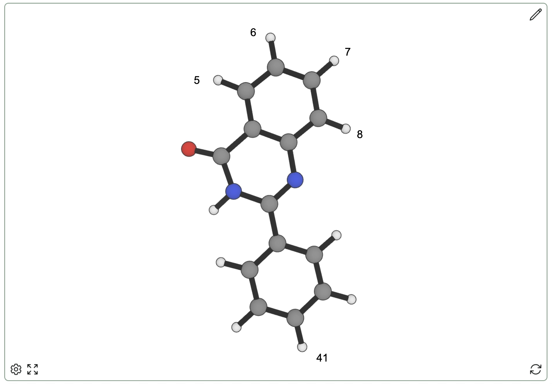
Ligand 1a from the Merck TNKS2 benchmark set with decoration sites labeled. We denote the phenyl para position as 41 and the four hydrogen-bearing positions on the quinazolinone benzene ring as 5–8.
Additionally, modes of generation differ substantially between models (see Appendix C). For example, some models only support decoration at pre-specified sites, others support looser decoration given a list of allowed sites, etc. This makes scaffold decoration hard to compare across models. In general, our experimental design goal was to let each model play to its strengths as much as possible, while restricting the final set of generated compounds to those which could reasonably be modeled by RBFE calculations.
We opted to use the Merck benchmark's ligand distribution over decoration sites and decoration site counts to inform parameter selection for the models that had parameters to select. For more exploration, we biased this distribution towards a flatter distribution over allowed combinations of decoration sites and decoration site counts. Details on how this was done are in Appendix D.
Loosely, we can characterize the generative parameters of the models as follows:
| Method | Site choice | Decoration size choice |
|---|---|---|
| LLMs | model | model |
| FLOWR | model | imposed |
| CReM | imposed | model |
| REINVENT 4 | imposed | model |
| DiffDec | imposed | model |
Pre-RBFE Results
At a high level, pocket-conditioned binder design aims to create new binders which match a given pocket. One implication is that the binders should actually fit inside the pocket and not e.g. incite dramatic steric clashes with pocket residues. To assay this, we required that all ligands have negative docking scores and MM/GBSA values—this criterion is relatively permissive, aiming only to exclude catastrophically bad ligands from downstream runs.
As anticipated, pocket-aware methods did not struggle here. Both FLOWR's and DiffDec's first 32 ligands to satisfy the structural constraints all had negative docking scores and MM/GBSA values. This is reassuring since both methods are pocket-conditioned. On the other hand, the non-pocket-aware method CReM struggled here: out of 50 generated, structural-constraint-satisfying ligands, only 29 met the docking criterion. So, we generated 10 more ligands—of which 6 were valid—and added the first 3 (in order of generation) to the existing set of 29. REINVENT 4 was a lot better, with 46/50 structural-constraint-satisfying ligands meeting the docking criteria.
Both LLMs tested performed very well here! GPT-5.6 Sol's first 32 molecules satisfied every single constraint. The worst docking score was −5.91, and the worst MM/GBSA single point energy was −33.36 kcal/mol.
Claude Opus 5 struggled slightly with protonation—3 of its first 32 molecules didn't satisfy constraint 4—but this isn't really concerning, as pKa-prediction models aren't completely consistent. After asking Claude to generate 3 replacement ligands, every molecule docked comfortably: the worst docking score was −7.26, and the worst MM/GBSA single point energy was −37.13 kcal/mol.
RBFE Single-Attempt Results
Unless otherwise stated, all FEP calculations used hub-and-spoke graphs (with the parent ligand as the hub) and Rowan's "Recommended" TMD settings.
Distributional Data
The binding affinity distribution varies drastically per method.
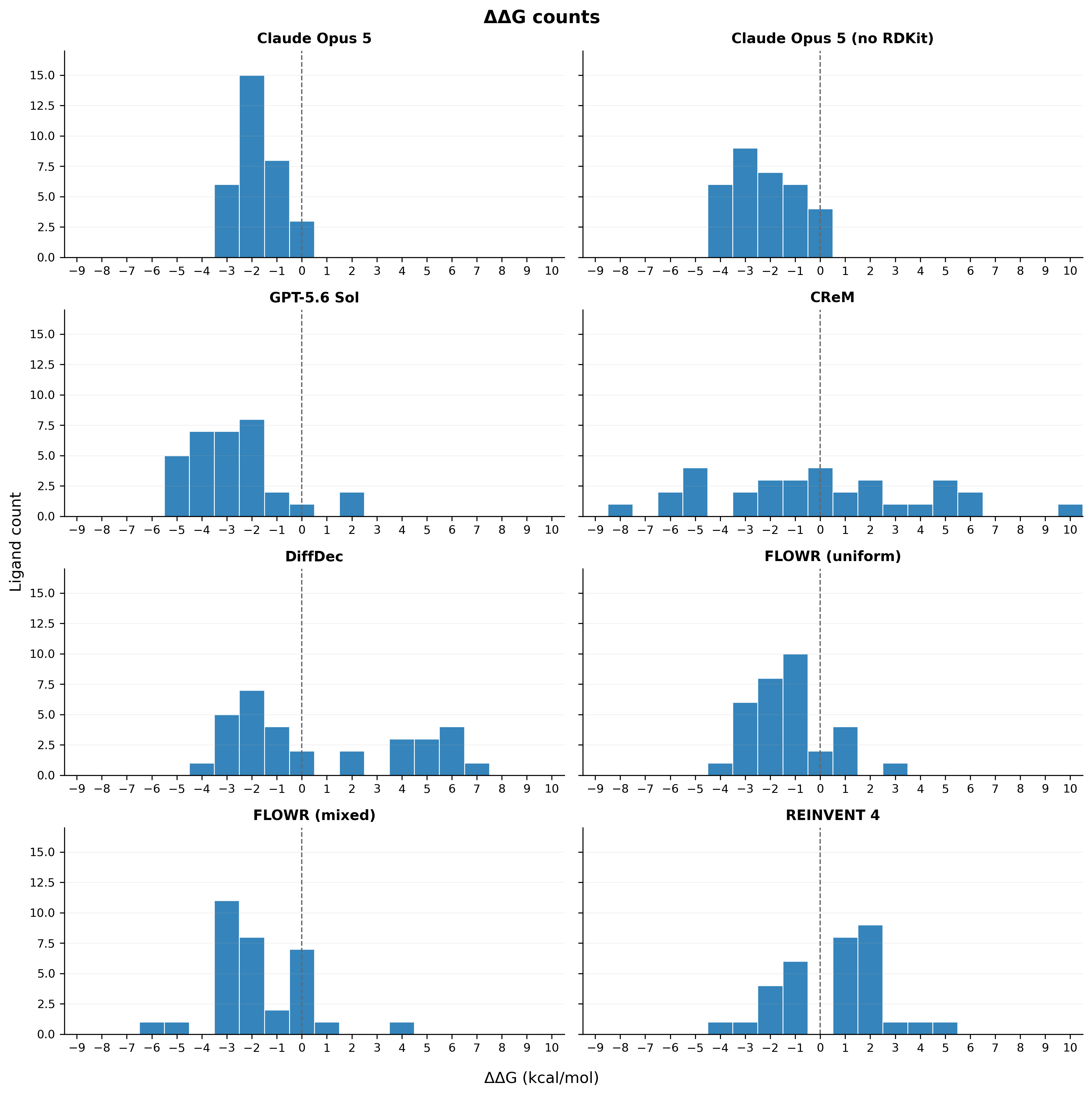
Single-attempt distributions. 32 constraint-satisfying molecules generated per method.
These results are pretty much expected. The pocket-aware methods, except for DiffDec, generally produce fewer ligands with positive ΔΔG values.
The failing ligands tend to place substituents at sterically constrained positions on the benzene ring, producing visibly strained pocket geometries and, in turn, unfavorable docking and MM/GBSA energies. In contrast, larger decorations pointing away from the pocket at the phenyl para position are generally favored. This suggests that DiffDec can perform poorly when asked to decorate sterically constrained sites.
It's also interesting to look at how big the decorations from each method are, as well as at which sites they tend to appear at.
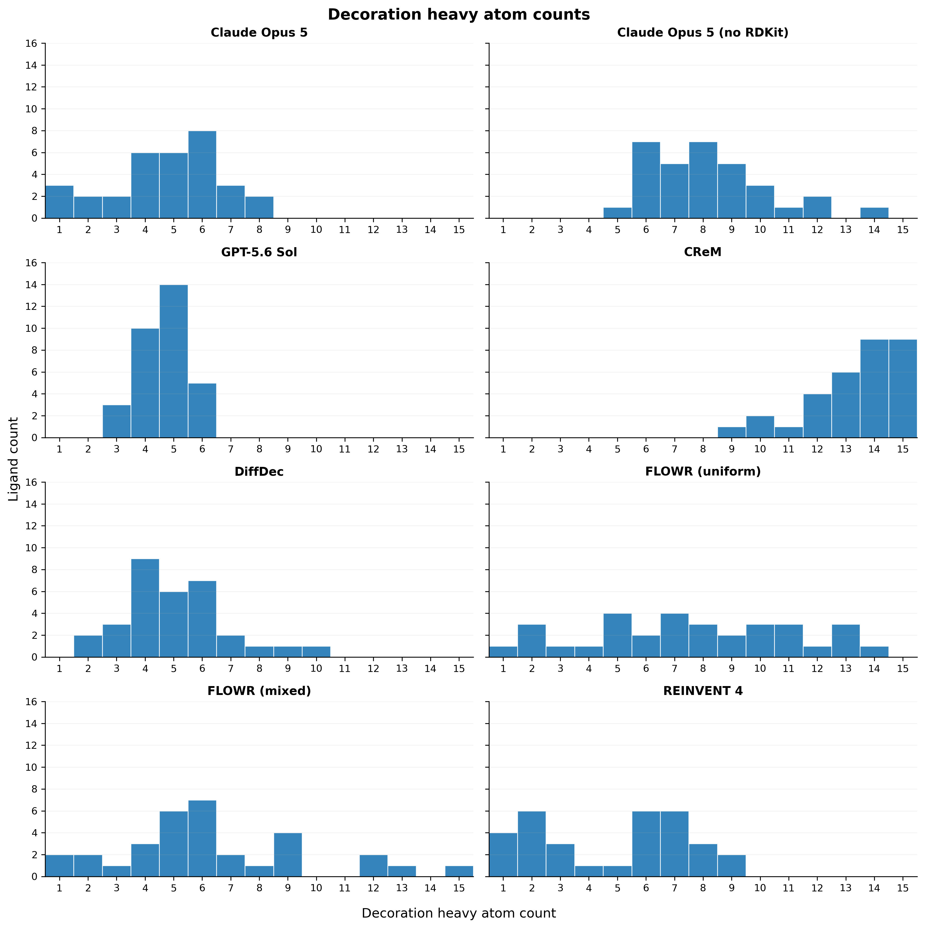
It's important not to read too closely into the distributional metrics for the models with lots of parameters, like DiffDec, since we chose the distributions for many of these parameters. With this in mind, even with the LLMs, we tend to see a lot of decoration strategies with a total of 4–7 heavy atoms.
FLOWR, however, is far more diffuse. CReM is the most clear outlier here, strongly favoring heavy decorations. Moreover, while this very well could be due to stochastic variation, we thought it was interesting that GPT-5.6 Sol's decoration heavy atom count distribution was much tighter than Claude Opus 5's.
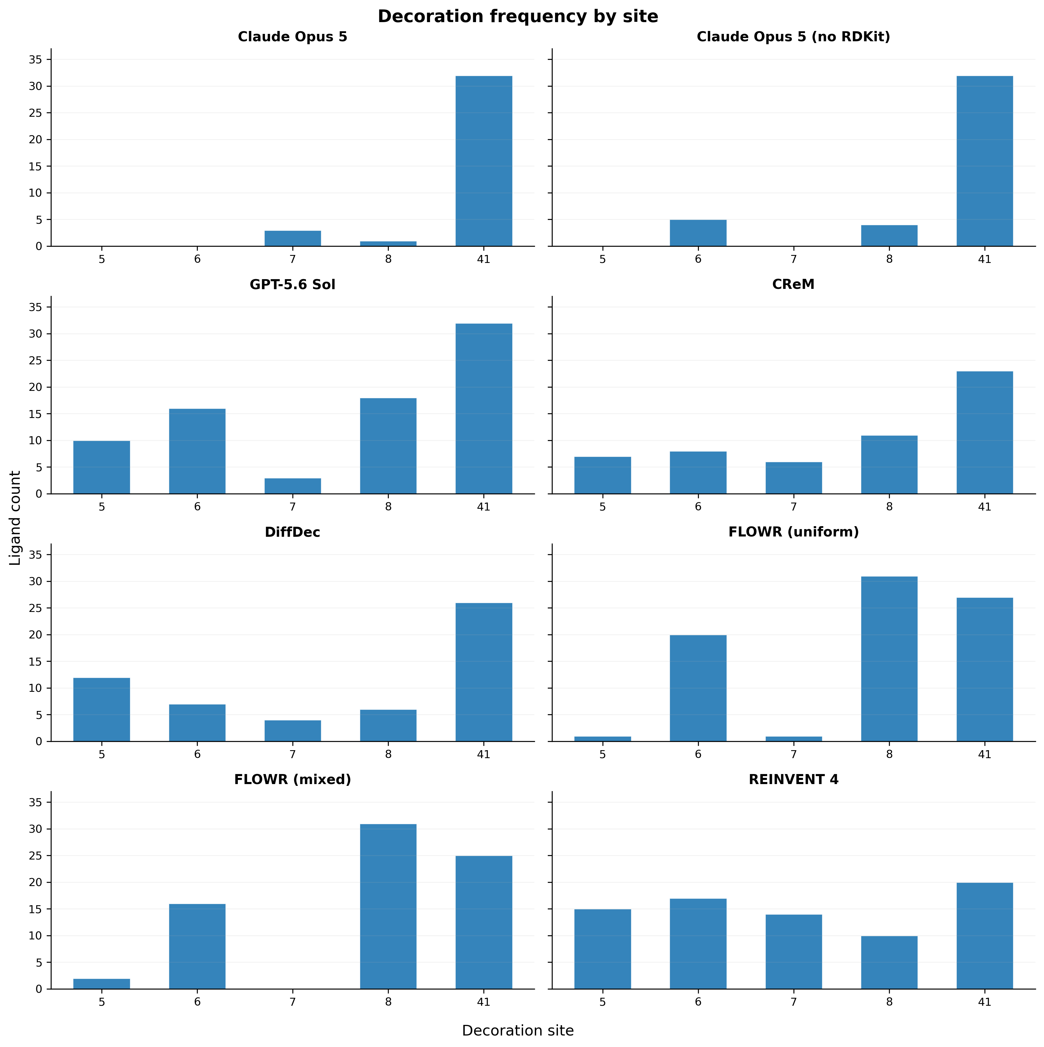
It is more informative to focus on FLOWR and the LLMs here, as they pick their generation sites. Site numbers are shown above in the first figure of this blog.
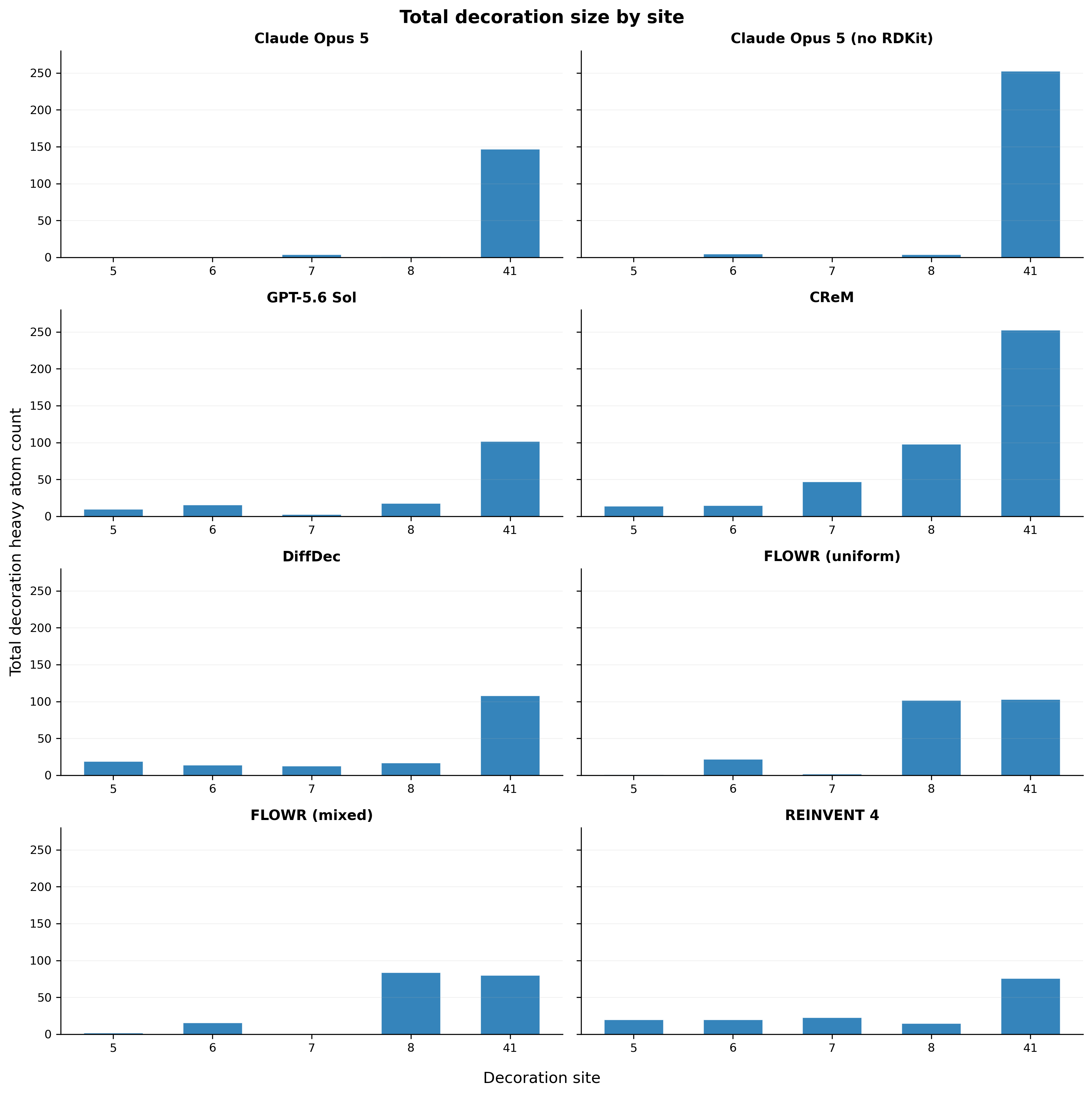
All models are informative here, though FLOWR has a set total decoration size (not by site!). This is relatively permissive, though. Site numbers are shown above in the first figure of this blog.
Across methods, most decorations are concentrated at site 41 (the phenyl para). This makes sense, especially since decorations here point outwards with respect to the pocket. Site 8 (on the quinazolinone benzene) is also a favorite, though taking the actual decoration heavy atom count per site into account demonstrates that the para decorations are much bulkier.
Top Binders
CReM dominated the tail of the single-attempt binding-affinity results, as is clear in the table below. All ΔΔG values are in kcal/mol with respect to the parent ligand. Binders stronger than −6 kcal/mol are highlighted in blue, binders between −6 kcal/mol and −5 kcal/mol are highlighted in green, binders between −5 kcal/mol and −4 kcal/mol are highlighted in yellow, binders between −4 kcal/mol and −3 kcal/mol are highlighted in orange, and the rest in red.
| Model | Rank 1 | Rank 2 | Rank 3 | Rank 4 | Rank 5 |
|---|---|---|---|---|---|
| GPT-5.6 Sol (High) | −5.437 | −5.093 | −4.703 | −4.688 | −4.579 |
| Opus 5 (High) | −3.219 | −3.106 | −3.062 | −2.884 | −2.823 |
| Opus 5 (High), no RDKit | −4.087 | −4.059 | −3.987 | −3.810 | −3.666 |
| CReM | −7.840 | −5.956 | −5.820 | −5.482 | −5.363 |
| REINVENT 4 | −3.987 | −3.020 | −2.453 | −2.401 | −1.691 |
| DiffDec | −4.182 | −3.277 | −3.175 | −3.040 | −2.880 |
| FLOWR.root (uniform dist.) | −4.337 | −3.498 | −3.409 | −3.374 | −3.332 |
| FLOWR.root (mixed dist.) | −5.996 | −4.904 | −3.382 | −3.370 | −3.289 |
For reference, the parent ligand has an experimental affinity of −8.55 kcal/mol.
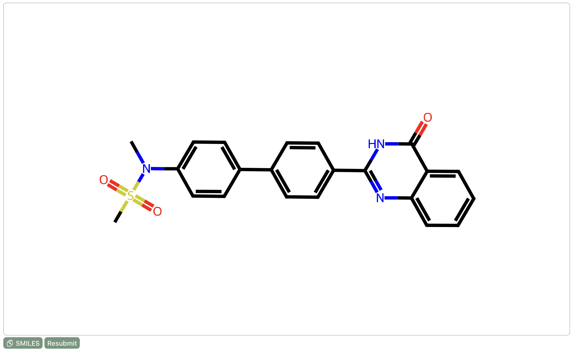
CReM and GPT-5.6 Sol clearly stand out, with all top 5 predictions sitting above the best binders from the reference data. Interestingly, their top designs differ substantially. The best CReM ligand is pretty beefy, with a single 15 heavy-atom decoration on the para position of the phenyl ring.
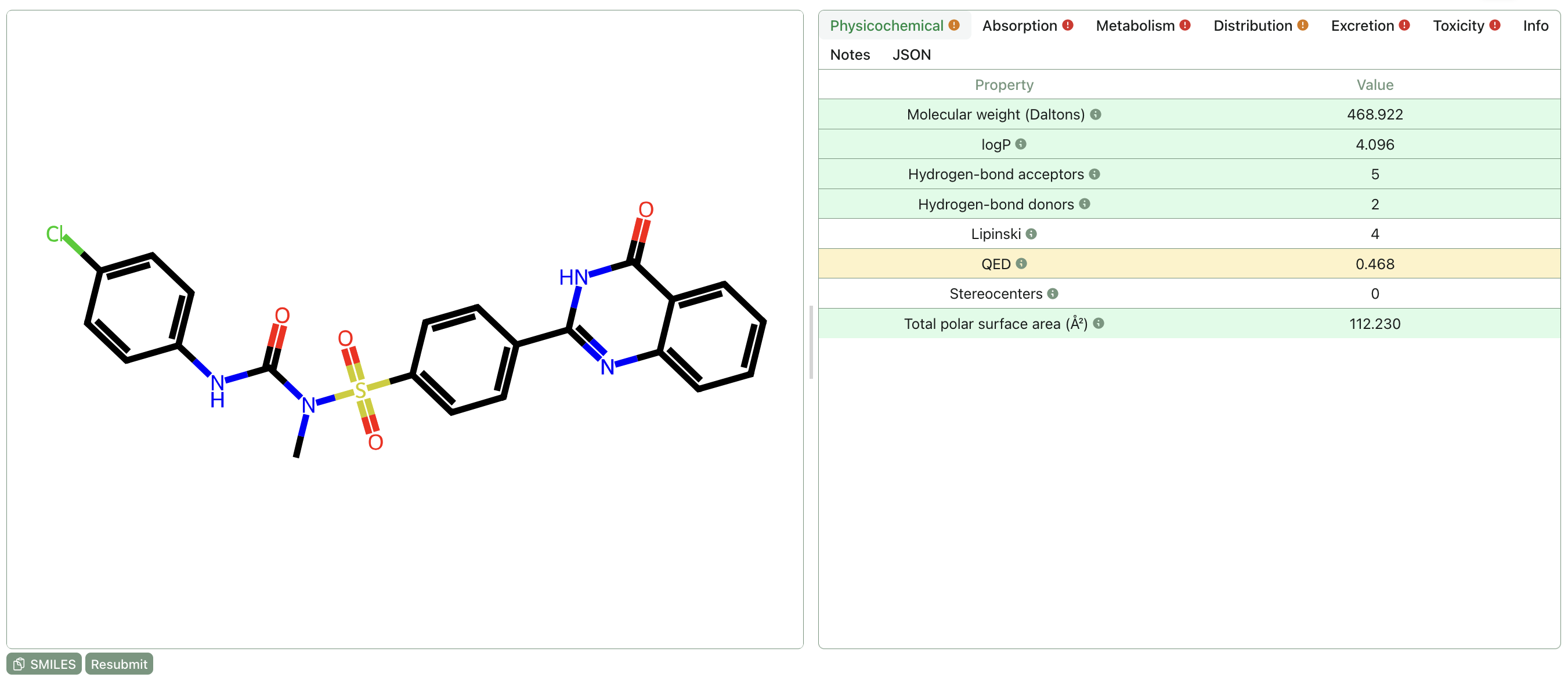
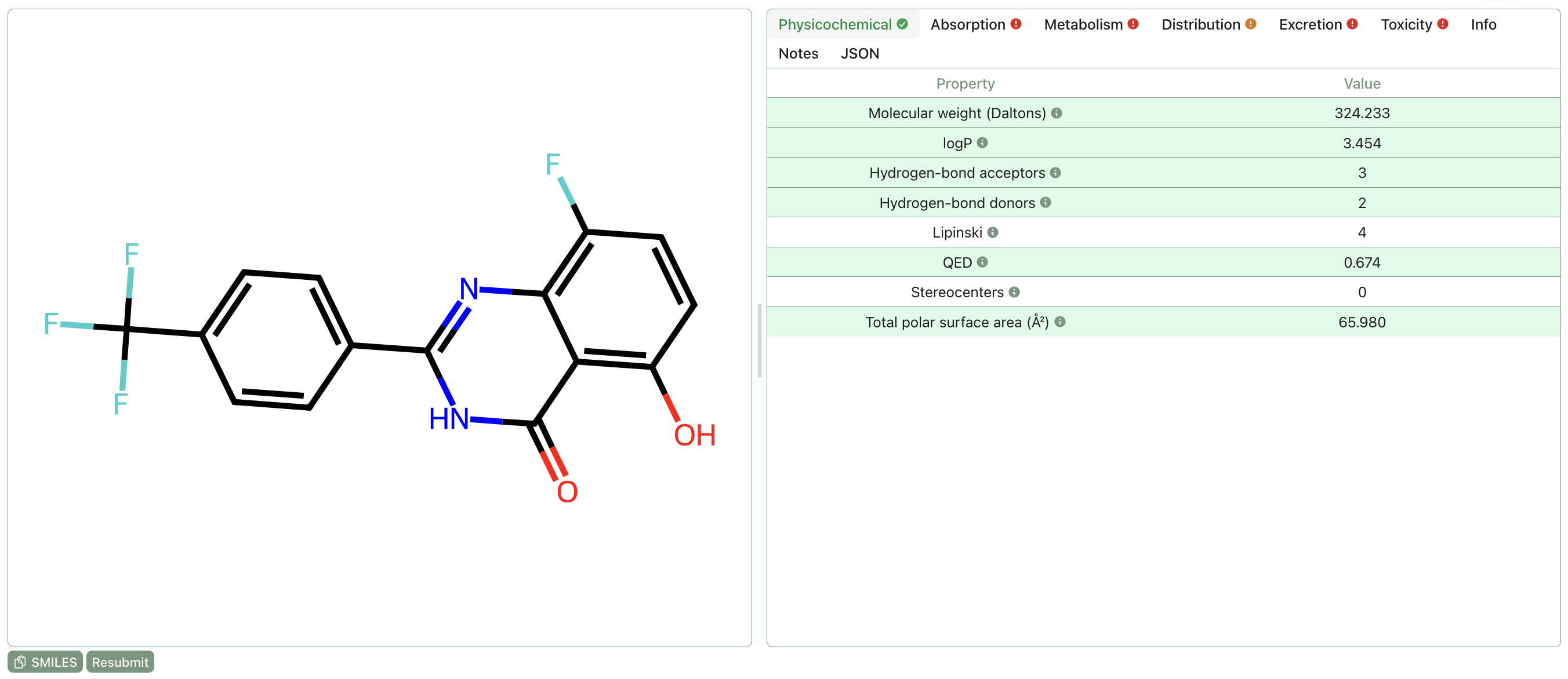
In contrast, the strongest GPT-5.6 Sol binder has decoration at 3 sites and is much smaller. It also has 4 fluorines, whereas the CReM binder has none. Broadly, this size trend holds among the top CReM and GPT-5.6 Sol binders: CReM's database favors heavier decorations on the phenyl-para, whereas GPT-5.6 Sol prefers to "sprinkle" much smaller decorations on several sites simultaneously.
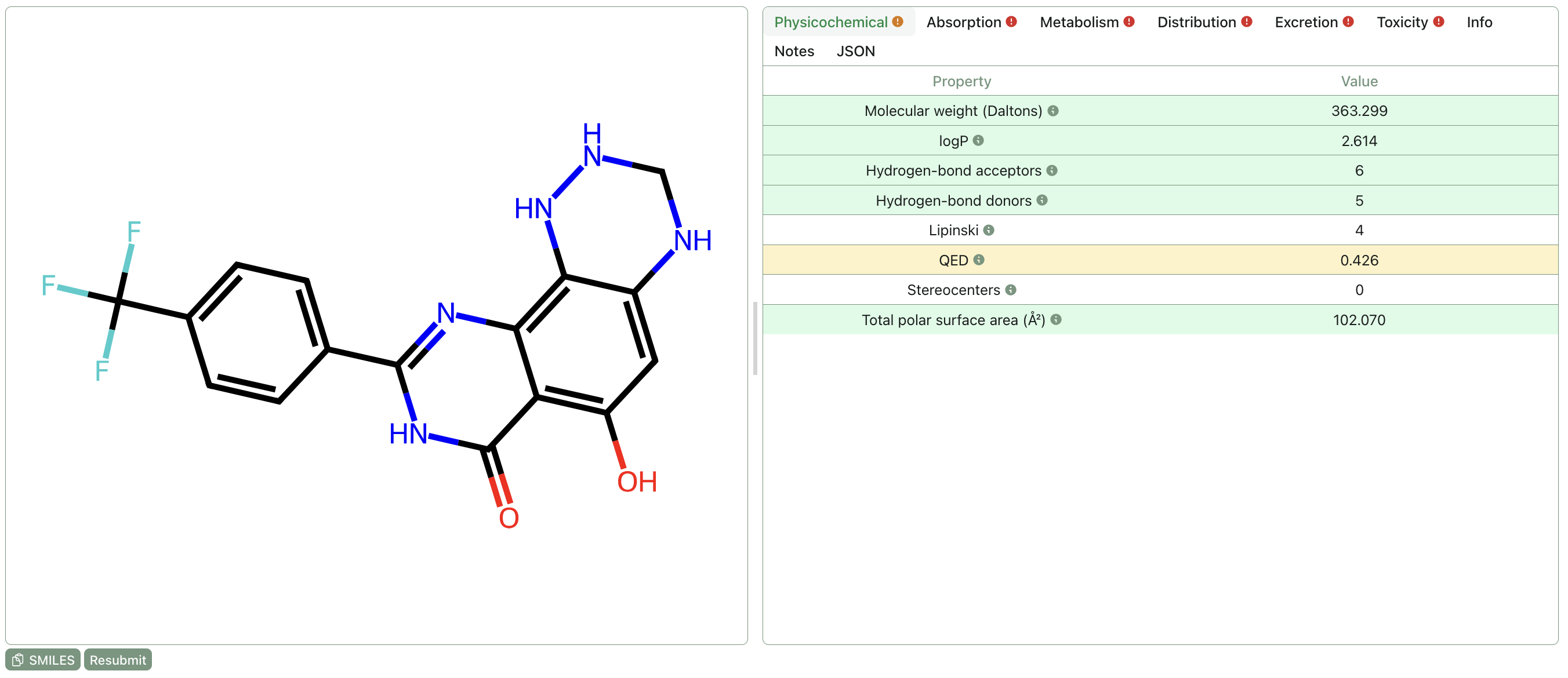
The top DiffDec compound contains a bizarre saturated triazacycle in combination with a trifluoro group on the phenyl. Other DiffDec runs reveal a penchant for similarly exotic functional groups, e.g. ring-fused azirines, hydroxylamines, or geminal diols.
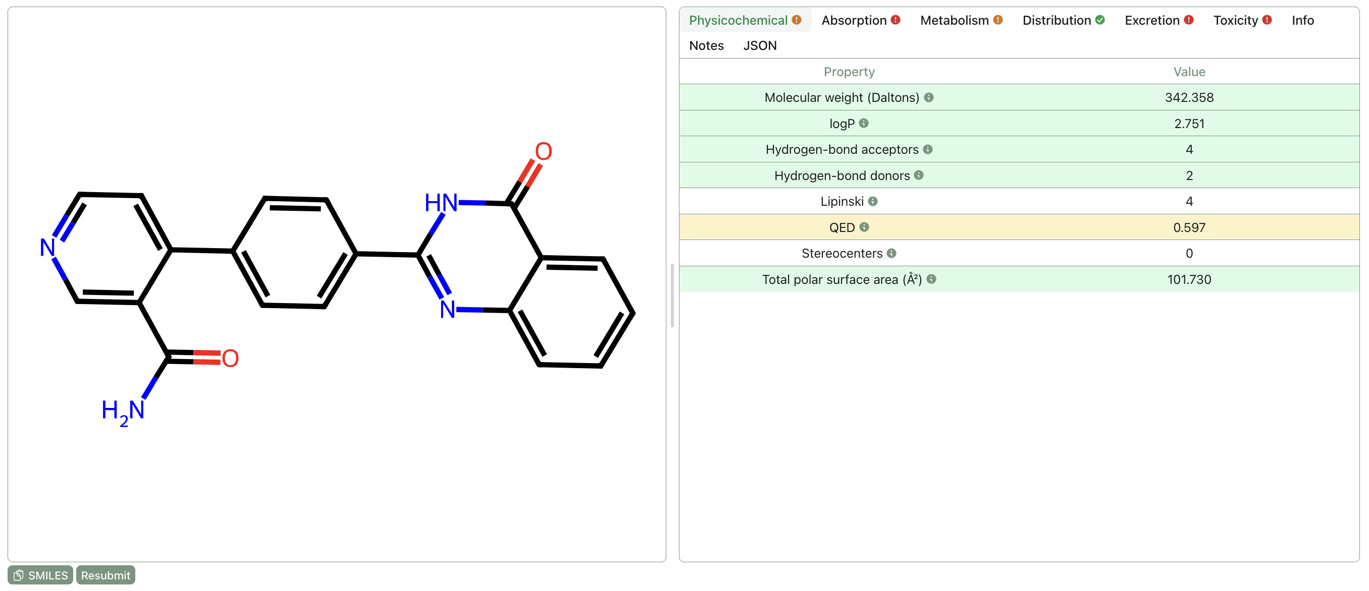
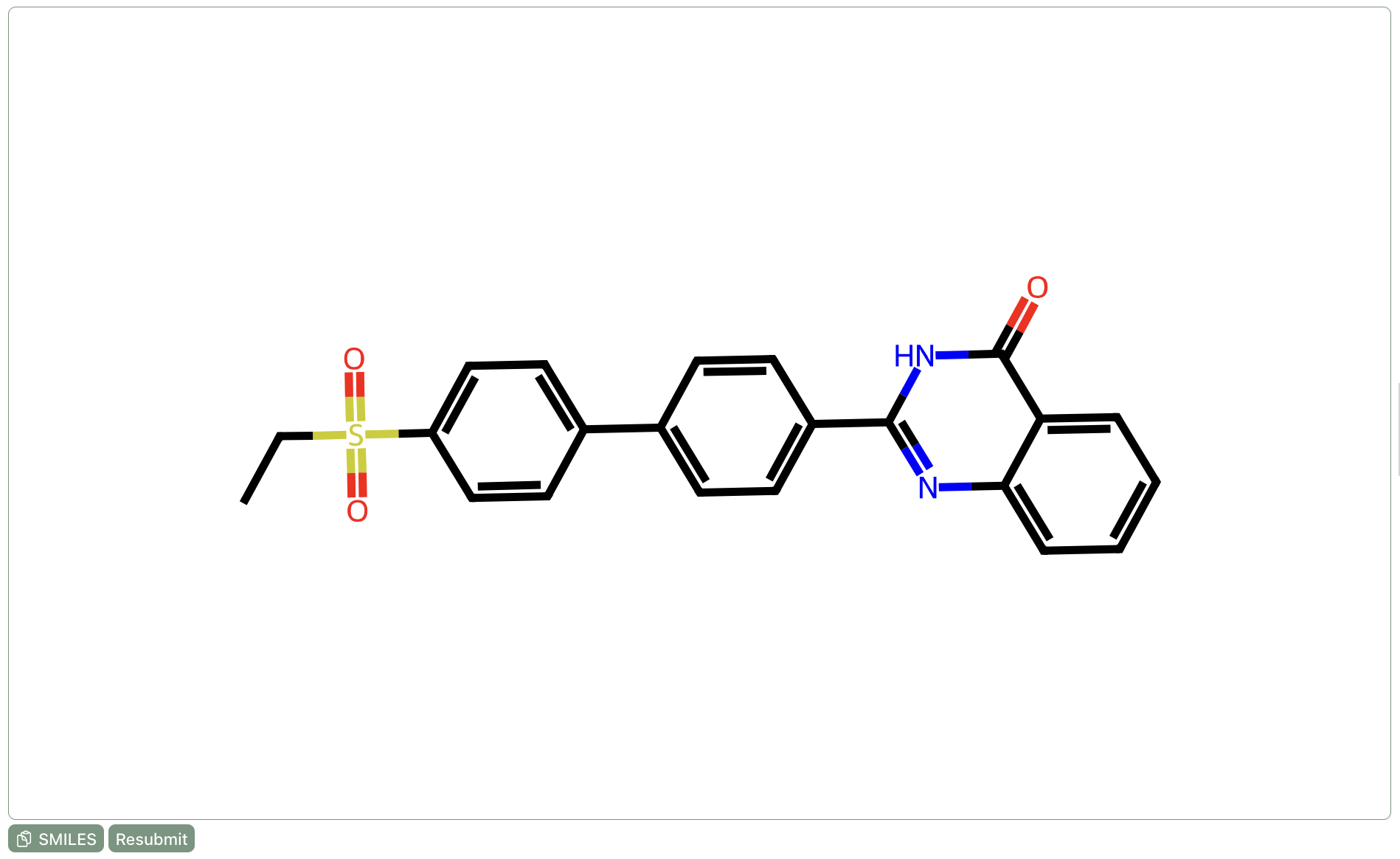
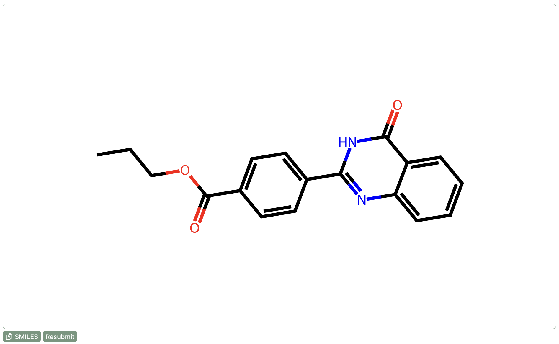
In contrast, REINVENT generally preferred relatively prosaic modifications—methylation, for instance, or addition of a pyridyl group at one site or another. The best REINVENT ligand fuses a nicotinamide to the para position of the ligand:
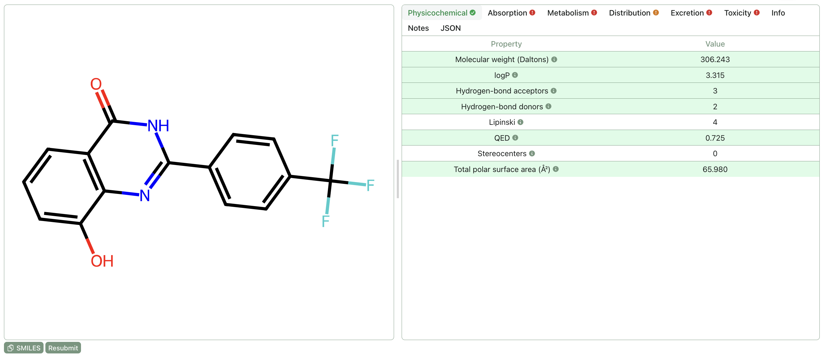
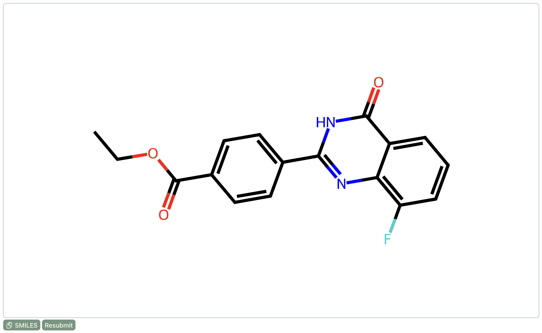
FLOWR, too, prefers small multi-site decorations, often featuring fluorinated groups like CF3 or OCF3. The best generated ligand from FLOWR combines a para-CF3 group on the phenyl with the addition of a phenolic oxygen to the quinazolinone core.
We can study the chemistry each model produces more broadly via a pairwise Tanimoto similarity matrix:
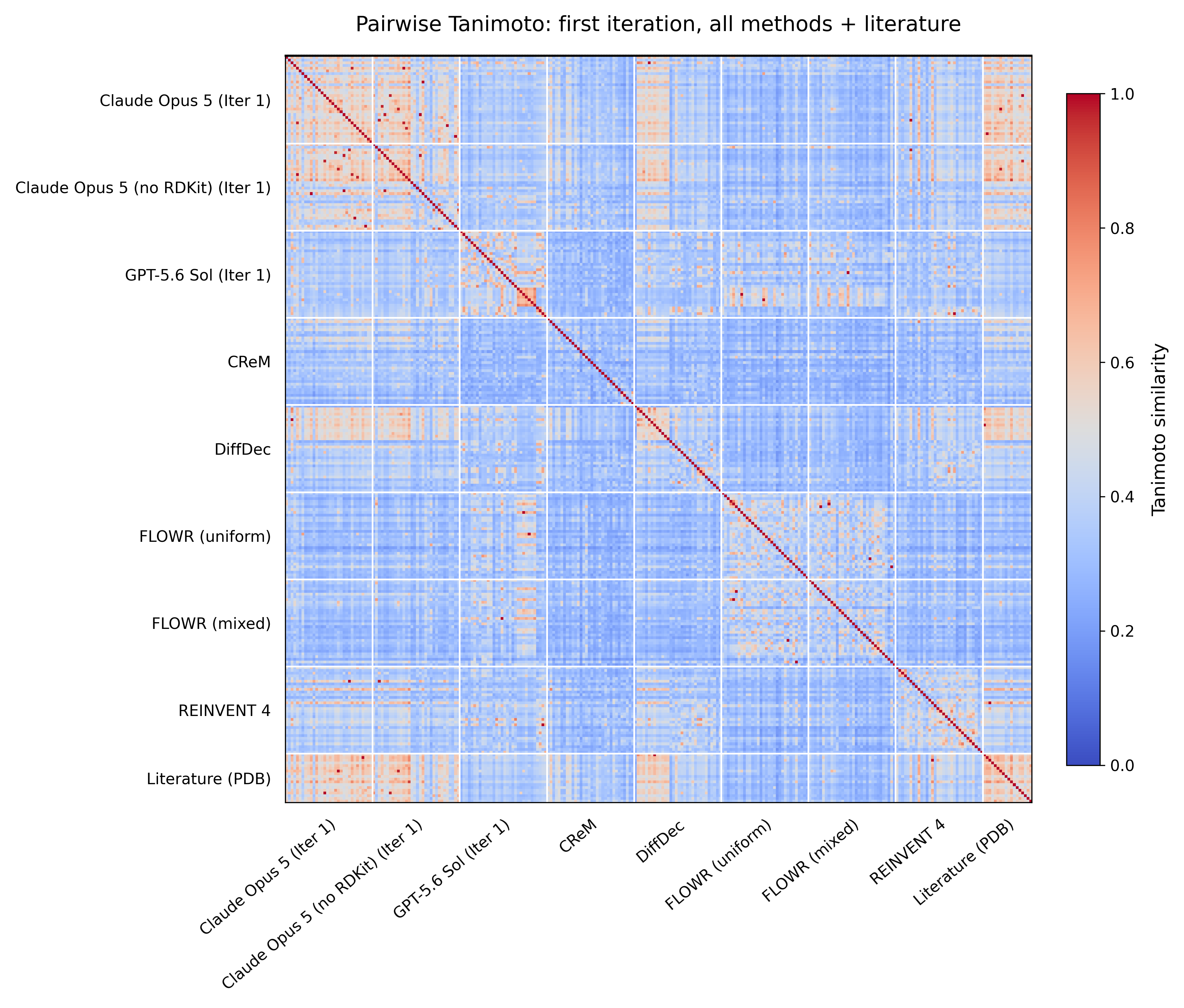
Within a method's "block," the generated ligands are sorted in order of binding affinity (excluding the literature results, which don't all have reliable binding affinities).
There's a lot to unpack here, but we thought it was particularly interesting that many of Claude's generated ligands are similar to one another and similar to the literature (TNKS2 inhibitors in the PDB). The best DiffDec binders are also similar to the best Claude binders (and, by extension, to many of the binders in the PDB). Barring a few pockets around the matrix, most molecules are pretty distinct from one another, at least per Tanimoto similarity.
RBFE Iterative Results
As is well described in other works (i.e. this work by Genentech), LLMs have the unique ability to iterate based on heterogeneous feedback without requiring a bespoke optimization procedure. This yields substantial gains on tasks that are, loosely, easy to "score" but hard to actually solve. We explored this approach by giving GPT and Claude the results of their previous RBFE, docking, and MM/GBSA runs to produce a new, unique batch of 32 ligands. See Appendix E for prompt information.
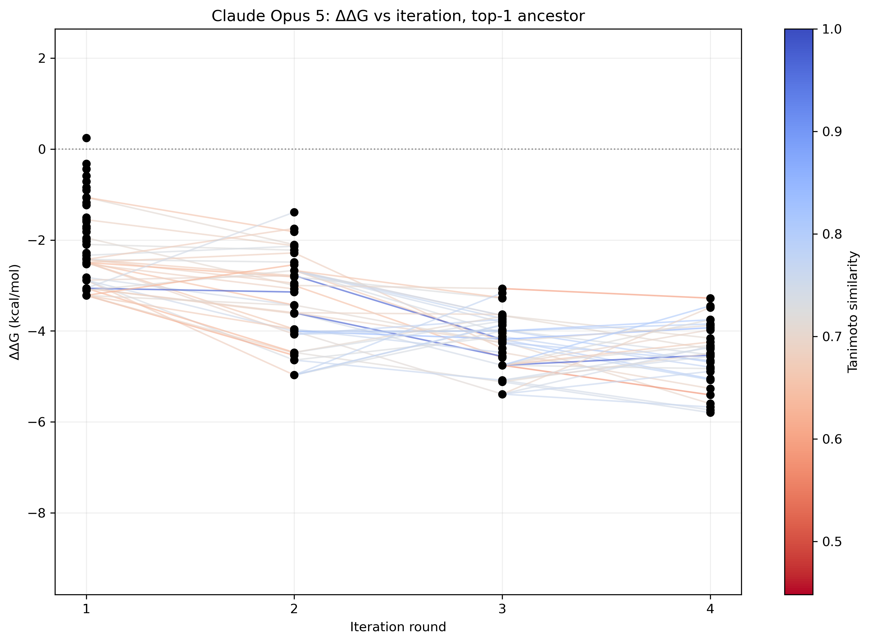
Notably, both models demonstrated unambiguous improvement over 4 iterations! Consider the top 5 binding affinities (kcal/mol) per iteration for both models:
| Model | Iteration 1 ΔΔG | Iteration 2 ΔΔG | Iteration 3 ΔΔG | Iteration 4 ΔΔG |
|---|---|---|---|---|
| GPT-5.6 Sol (High) | 1. −5.437 2. −5.093 3. −4.703 4. −4.688 5. −4.579 | 1. −7.957 2. −7.720 3. −7.507 4. −6.860 5. −6.782 | 1. −8.582 2. −8.192 3. −8.192 4. −8.157 5. −8.121 | 1. −9.232 2. −9.117 3. −8.870 4. −8.856 5. −8.634 |
| Claude Opus 5 (High) | 1. −3.219 2. −3.106 3. −3.062 4. −2.884 5. −2.823 | 1. −4.970 2. −4.641 3. −4.539 4. −4.486 5. −4.473 | 1. −5.388 2. −5.119 3. −5.084 4. −4.754 5. −4.587 | 1. −5.796 2. −5.738 3. −5.673 4. −5.599 5. −5.406 |
The improvement over iterations is so strong with GPT-5.6 Sol that every single top-5 binder in a future iteration binds more tightly than all binders in previous iterations! Such improvement is also unambiguous in Claude's design campaign, albeit a little less substantial.
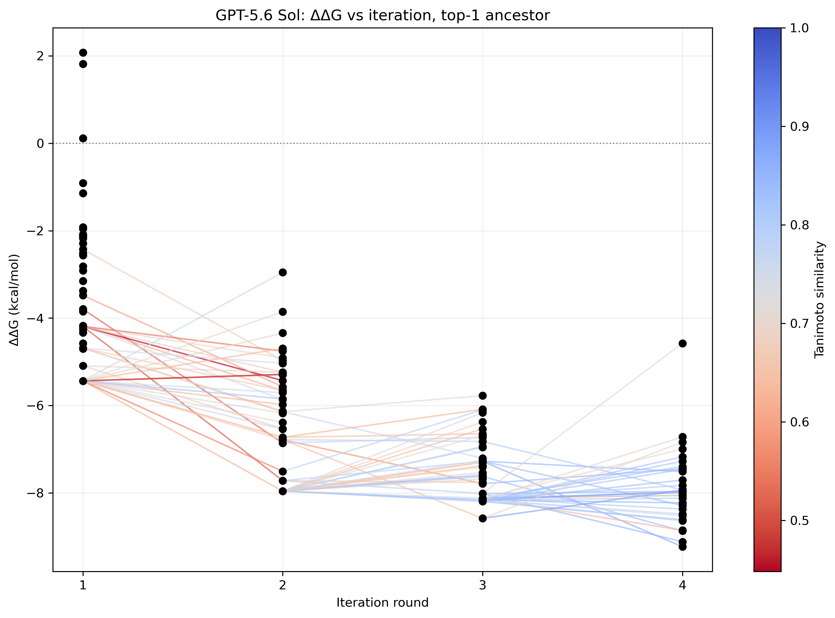
A line joining a ligand X from iteration T to a ligand Y in iteration T+1 indicates that ligand X is the most similar ligand out of all of the iteration T ligands to ligand Y. The line's color indicates Tanimoto similarity.
GPT-5.6 Sol's search heuristic is interpretable. As the model iterates, the model explores fewer chemical neighborhoods and concentrates on the few that have already produced strong TNKS2 binders. Early rounds have large ΔΔG spreads and large chemical jumps between iterations; later rounds are dominated by smaller chemical changes to the existing best binders. In the above plots, this can be visualized through the Tanimoto similarity to the closest parent compound. Early on, each new compound is highly dissimilar to previous compounds; towards the end, most ligands have high similarity to an already strong binder.
This "steering" that we get for free is really nice—with specialized models, there isn't always a clear way to do this. Different complex approaches could be envisioned: one could try to fix decorations at some sites and encourage generation at others, run unconstrained generation and filter based on an updating MCS, or do something else. It isn't obvious what the best approach is, and LLM generation avoids this altogether.
Opus 5's search isn't as clean as GPT-5.6 Sol's, though it adopts loosely similar search strategy in its exploration favoring perturbations of the strongest binders.
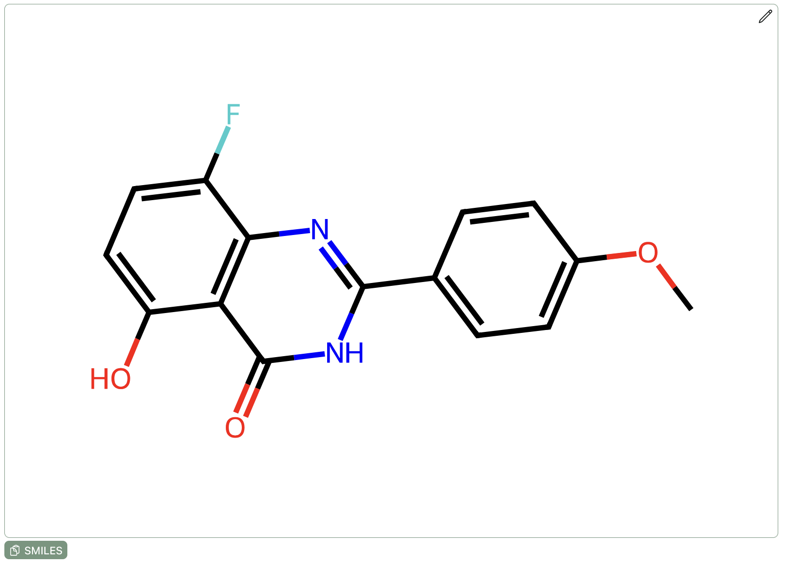
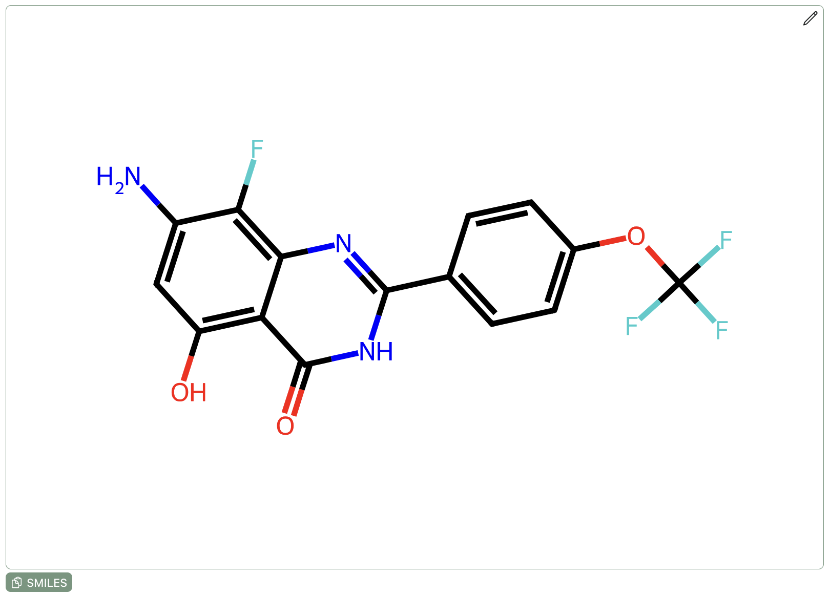
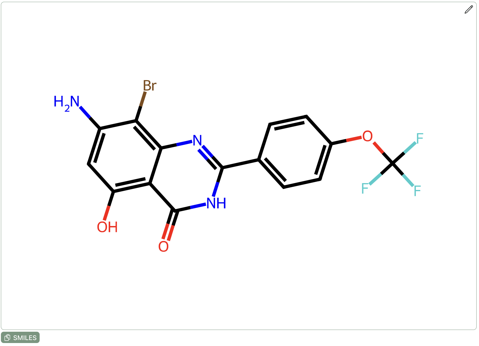
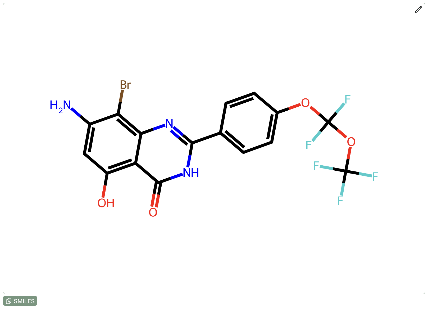
The above ligands form the "lineage" of the strongest GPT-5.6 Sol binder by the fourth iteration, obtained by tracing the path of edges from the bottom right point in the GPT-5.6 Sol plot back to the first generation. The steps taken between consecutive iterations are pretty apparent; the first step is probably the largest, with the addition of the amino substituent on the quinazolinone and the methoxy → trifluoromethoxy replacement. The scaffold is then pretty locked in, with more minor decorations via the fluorine → bromine replacement and the addition of a more complicated perfluoroether group.
Analyzing Properties of Generated Ligands
It's worthwhile to analyze the properties of the ligands produced by each of the models. There are loads of things to look at here: decoration site preferences, decoration motif preferences, logP values, heavy atom counts, etc.
As might be expected for a task focusing on growing a fragment into a better binder, most modifications substantially increase the heavy-atom count of the ligand. Not all modifications are created equal, though—while many models propose binders with 10 additional heavy atoms, GPT-5.6 Sol gains an additional −0.757 kcal/mol per heavy atom on average, while CReM gains only −0.092 kcal/mol per heavy atom on average. We feel that metrics like ligand efficiency can be useful in real medchem contexts (despite the controversy around them), but we chose not to emphasize these sorts of metrics here as the larger point of this work is to show that iteration with RBFE as an oracle works.
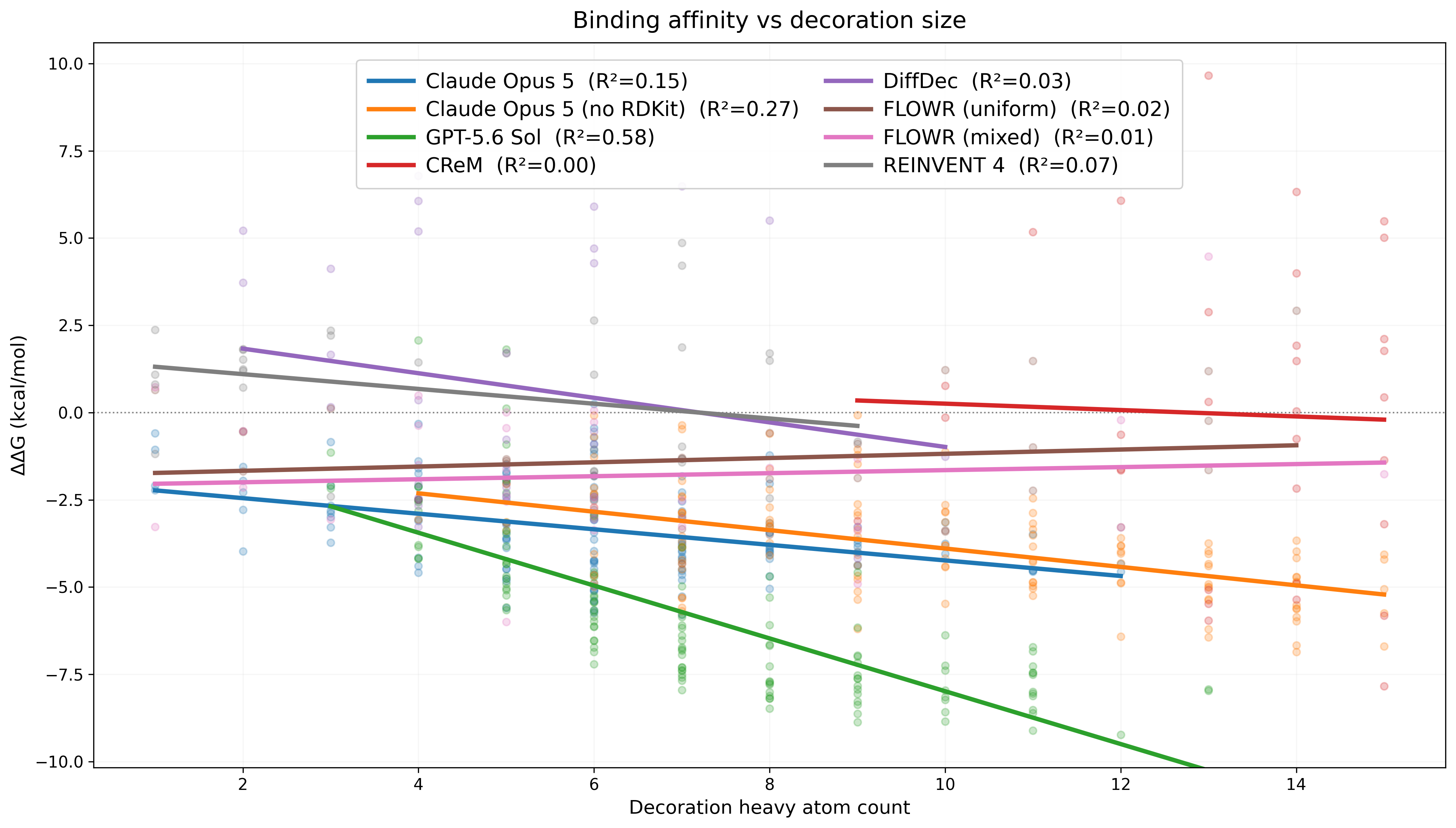
Bigger ligands produced by the LLMs generally bind more tightly, whereas decoration size and binding affinity are uncorrelated for the specialized models.
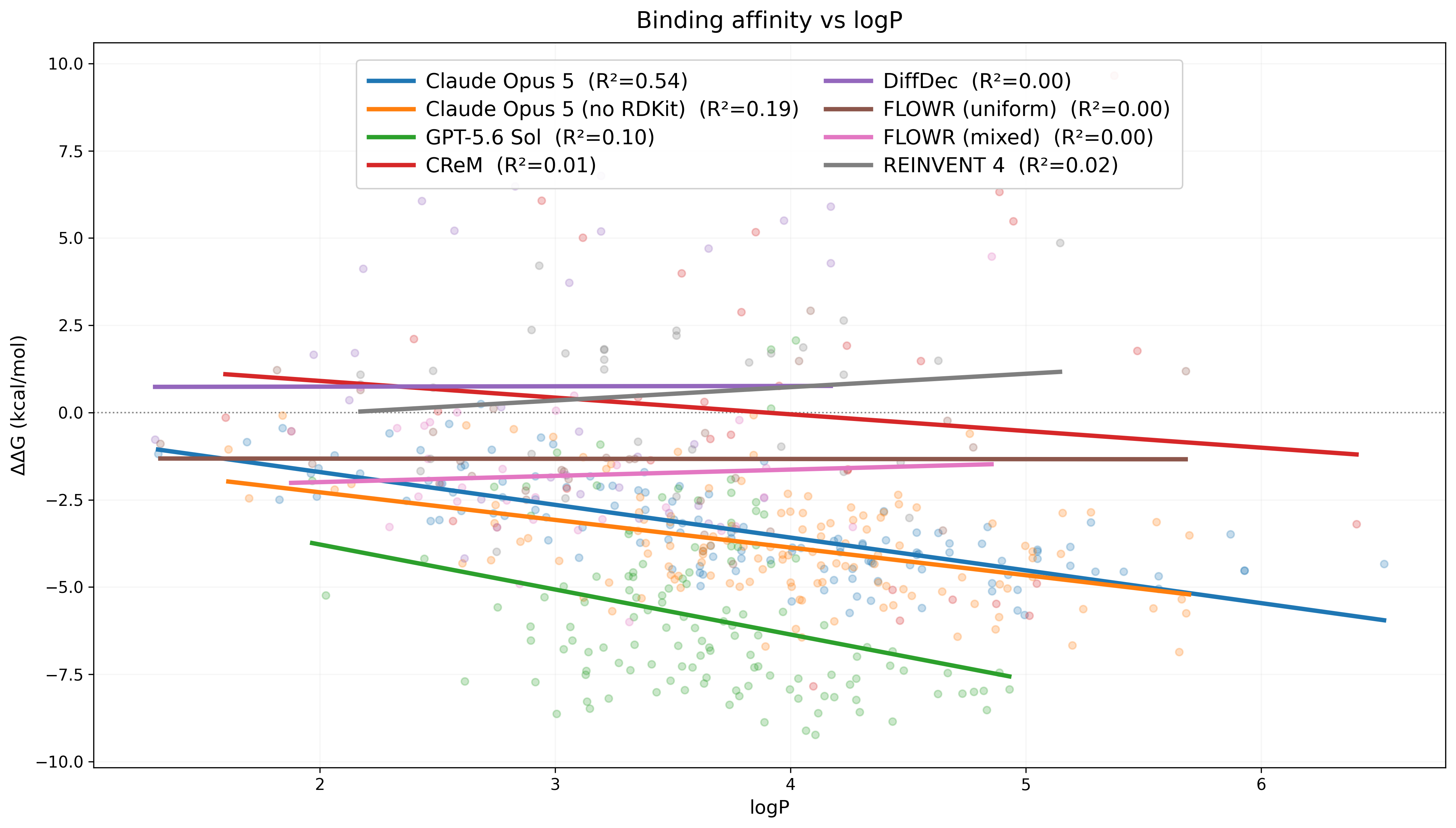
The LLMs exhibit correlations between logP and binding affinity. This plot features all LLM data across iterations, so iteration number is a substantial confounder here.
The correlations observed for the LLMs reflect a learned decoration strategy rather than a generic preference for large or lipophilic ligands. Over iterations, both LLMs are partial to hydrophobic, generally heavily fluorinated substitution at the phenyl para site. This is especially true for GPT-5.6 Sol, which evolves from smaller substitutions to larger ones. Opus 5 reaches similar but more compact substitutions.
Also, the specialized models don't exhibit the same correlations that the LLMs do, highlighting the importance of substituent placement and chemistry.
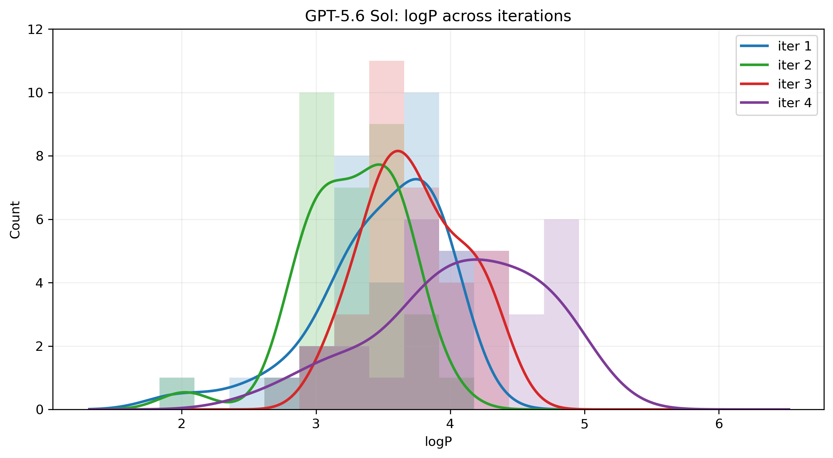
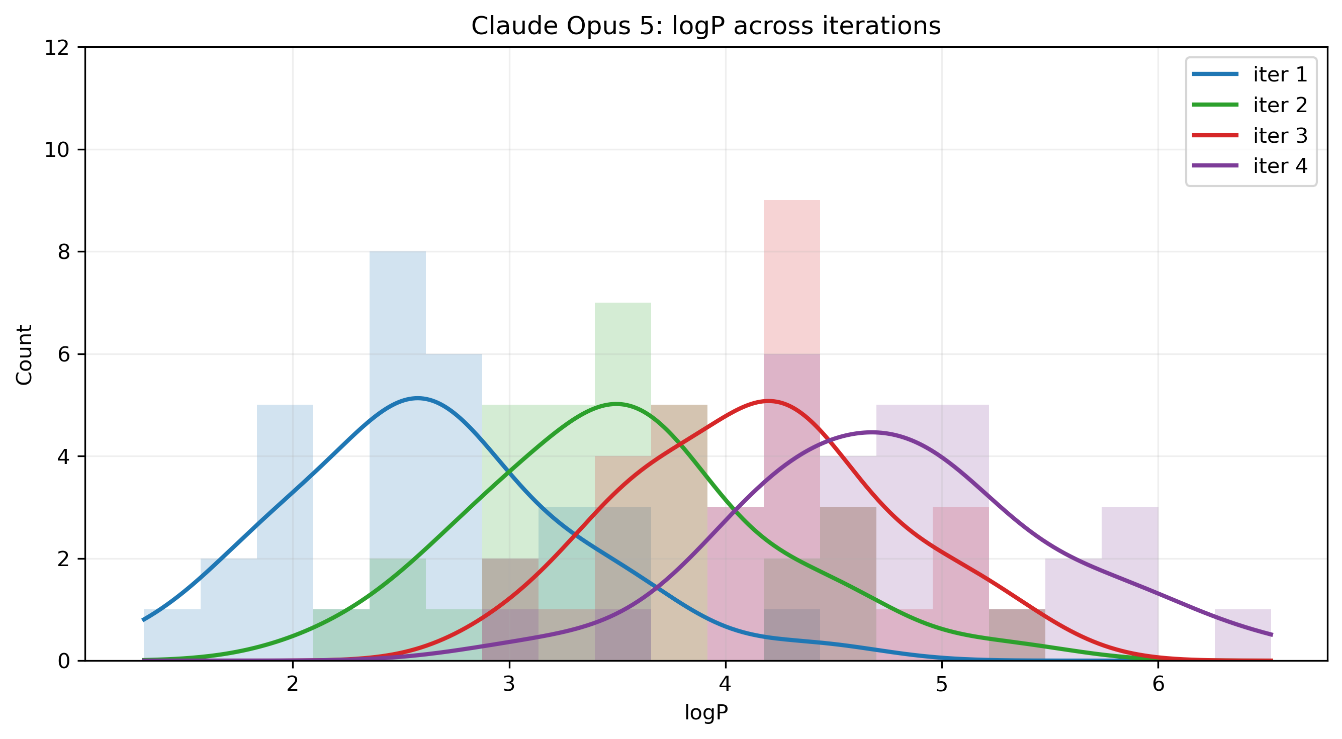
Claude's molecules become clearly more lipophilic across iterations.
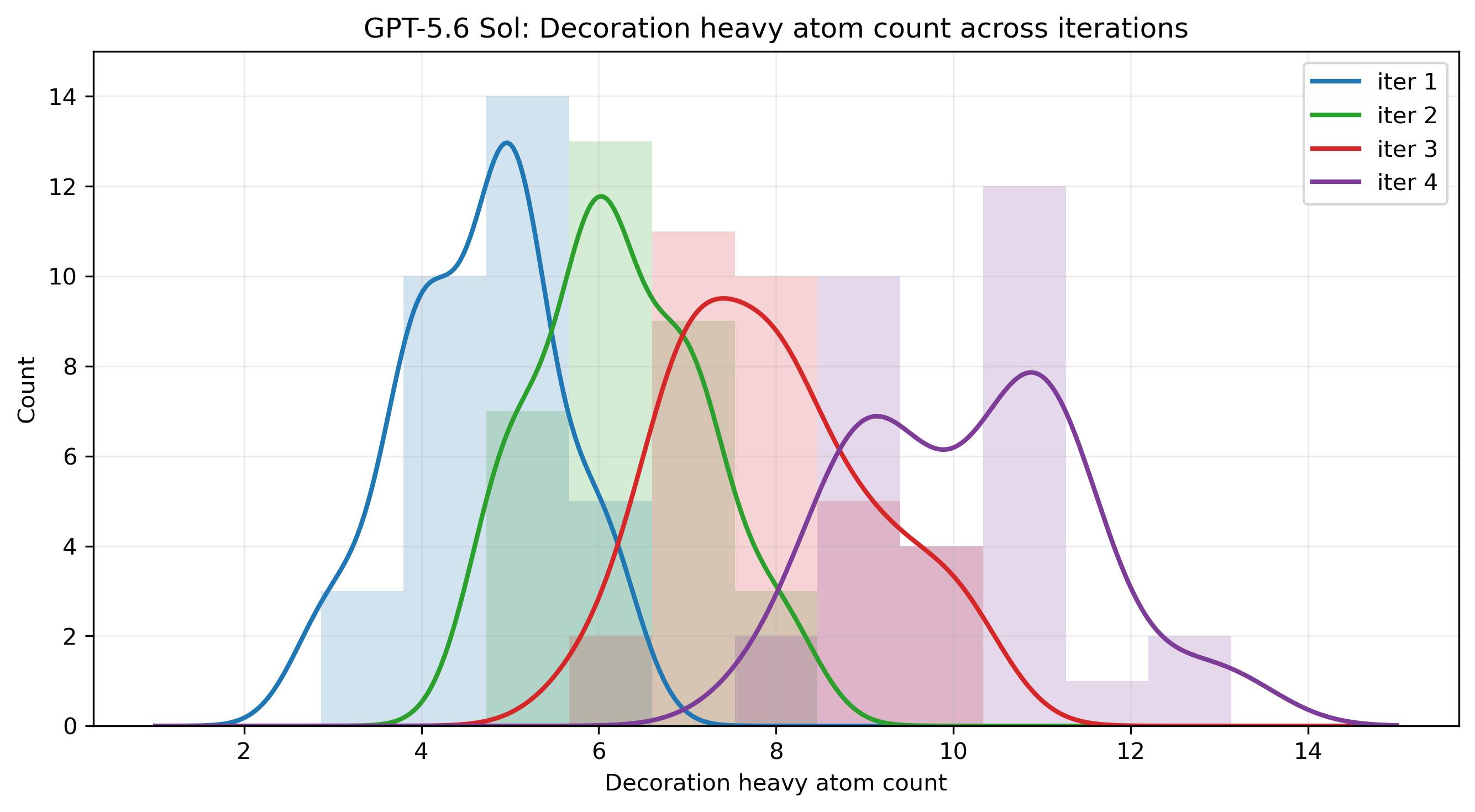
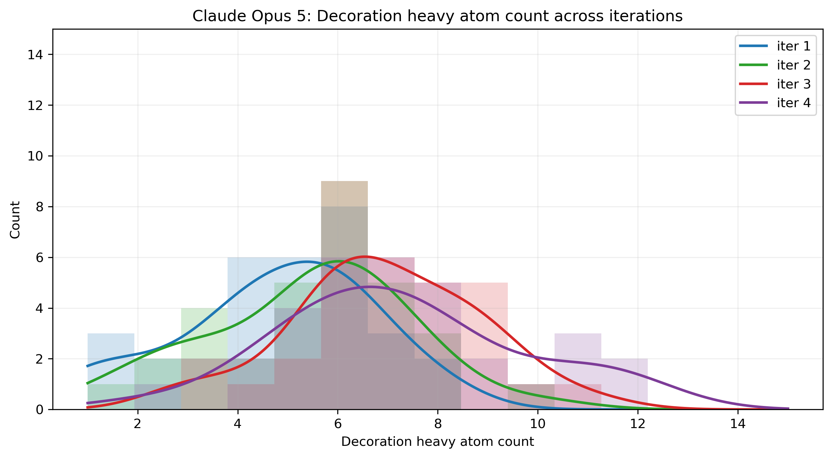
Claude decoration sizes are pretty diffuse, but it starts pushing towards larger ligands in later iterations.
The property distributions across iterations make the LLM optimization trajectory explicit. Both models progressively explore larger ligands while simultaneously veering into higher-logP chemical space. These plots, in conjunction with the ancestry plot, show that the models have pretty good exploration/exploitation reasoning.
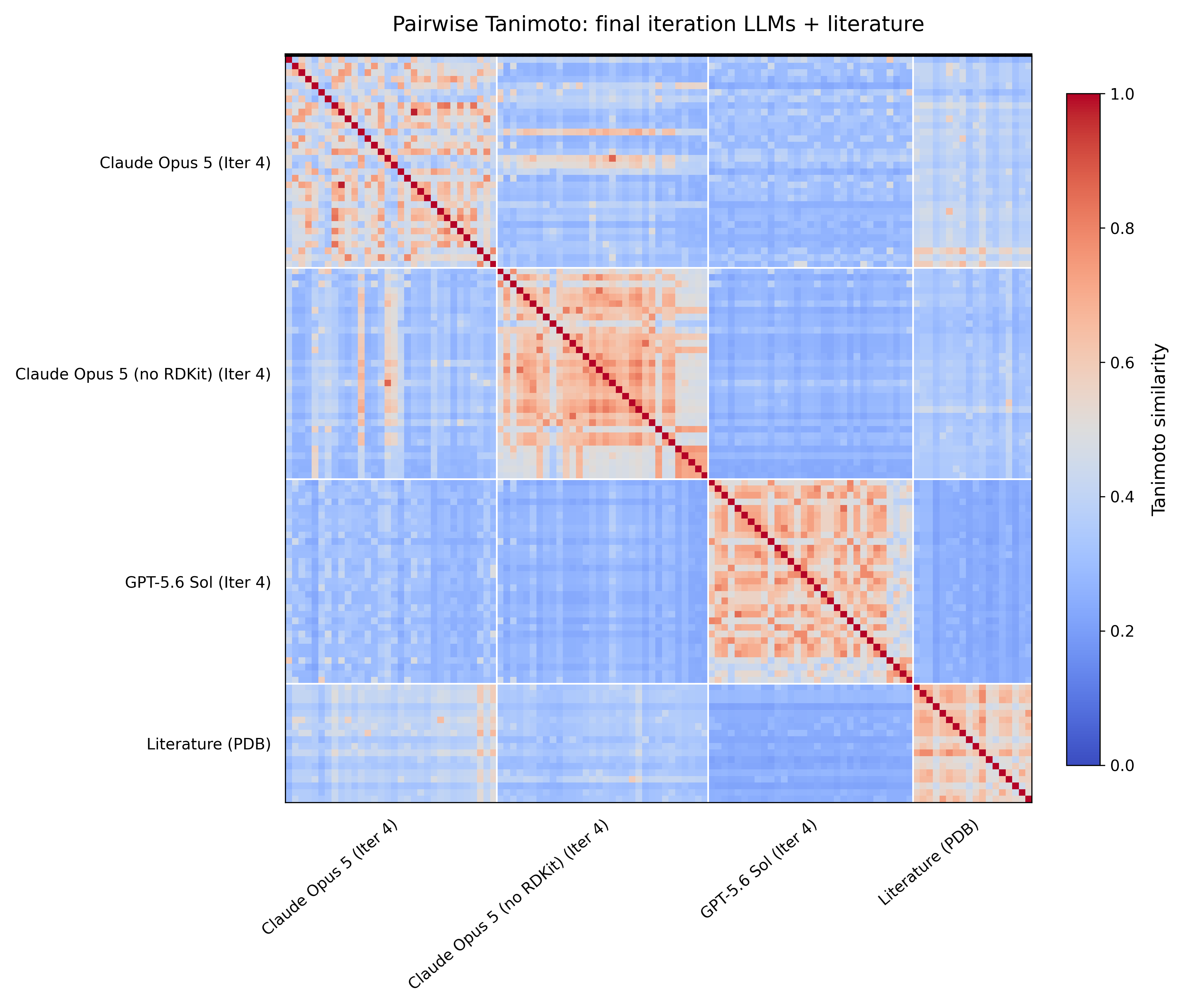
The results are generally quite disjoint from the PDB inhibitors, suggesting that LLMs explore new regions of chemical space and haven't simply memorized literature precedent.
Pocket Sensitivity Controls
As far as we can tell, the strongest binding ligands produced by the LLMs haven't been studied much in the context of TNKS2 (see above pairwise heatmap). Despite this, we think it is important to run controls on the LLMs to ensure that there isn't any "cheating" occurring. Recent work shows that co-folding models can predict nearly identical binding poses even upon drastic pocket modification, which suggests pervasive pocket memorization. To rule out a similar pathology here, we perform a single-residue mutation to validate that different pockets lead to different generated ligands.
For this study we perform a single-site mutation at residue 85, originally a phenylalanine, by replacing it with a glutamine.
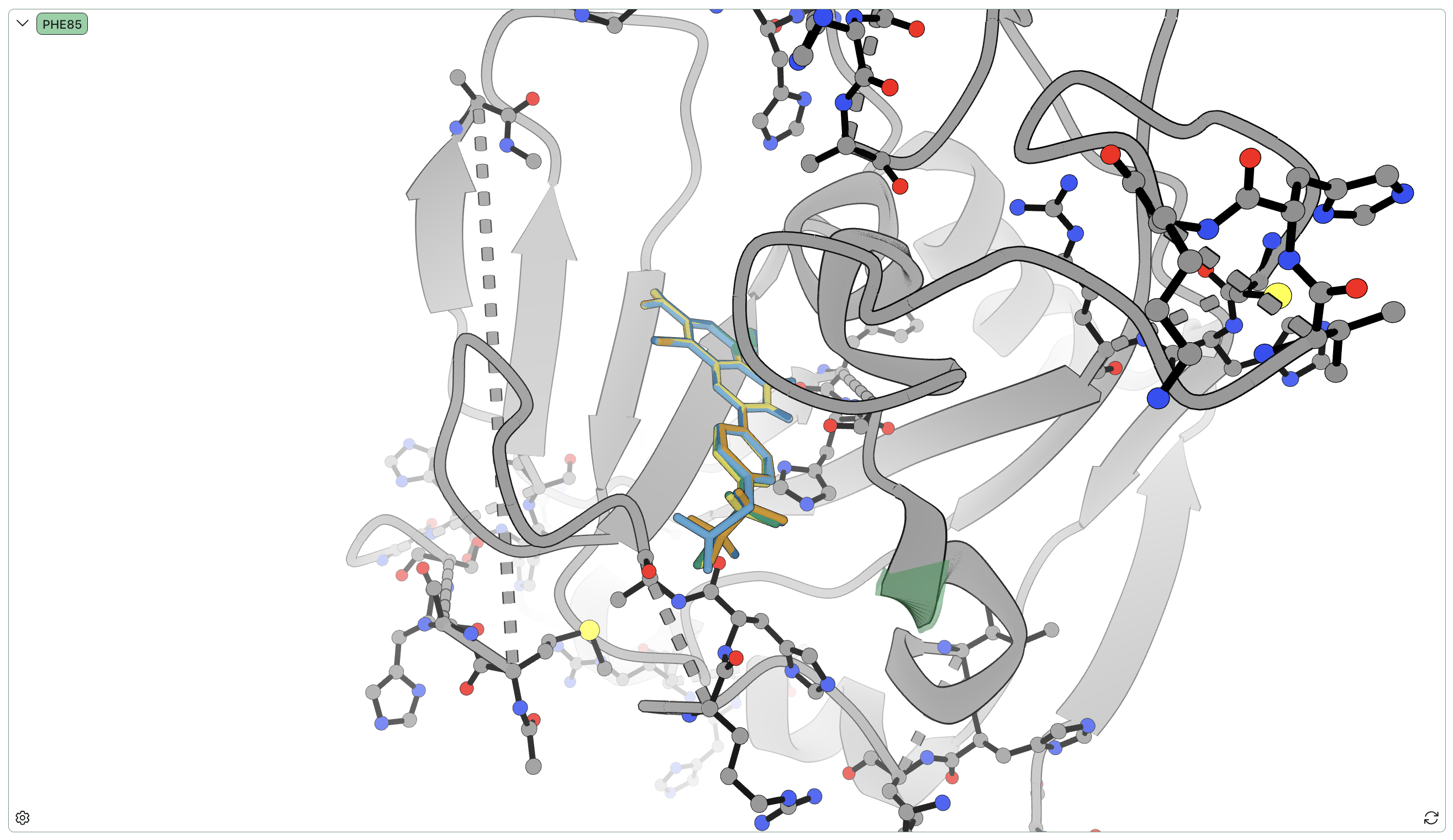
Docked poses for the eventual top five GPT-5.6 Sol ligands after three iterations.
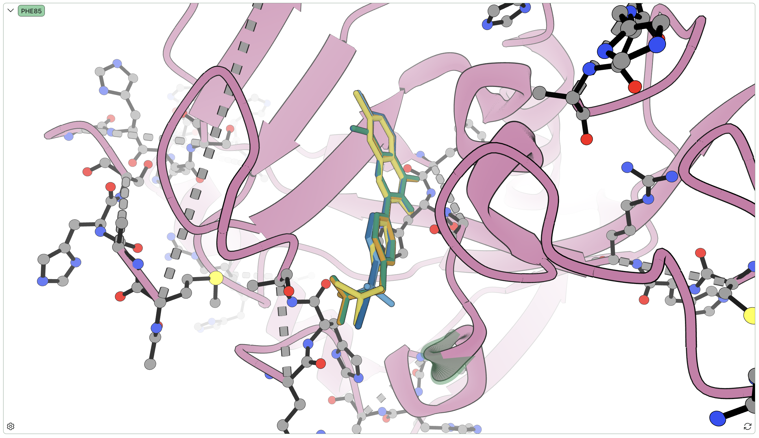
Docked poses for the eventual top five Opus 5 ligands after three iterations.
Our thought process was as follows: most LLM-produced decorations put something on the para—as is pictured in the above images—and the phenylalanine is adjacent to these decorations. Thus, switching the phenylalanine for something chemically dissimilar (polar instead of nonpolar, hydrophilic instead of hydrophobic, etc.) should yield meaningfully different predictions from LLMs. Glutamine fits these constraints well.
After making the glutamine substitution, we ran a short MD relaxation of the mutated receptor complexed with the parent ligand to get a physically reasonable receptor geometry, akin to induced-fit docking. Then, we followed the exact same iterative LLM-decoration procedure for a single iteration (totaling 64 ligands generated per LLM).
The ligands generated in the mutant F85Q pocket are different than the ligands generated in the wild-type pocket. In all three wild-type cases, the best binders by the second batch of generated ligands tend to have fluorine decorations on the para. However, in the mutated cases, the strongest binders have no fluorine on any para decoration.
In fact, almost none of the F85Q ligands have fluorinated decorations at site 41. 24/32 GPT-5.6 Sol ligands and 18/32 Claude Opus 5 ligands have fluorinated para decorations by the second iteration provided the wild-type pocket. These fractions plummet to 1/32 and 4/32 (respectively) when given the mutated pocket, indicating that the LLMs aren't merely using memorized results from the literature.
RBFE Robustness Check
The imposed MCS constraint featured in this benchmark lends itself to a hub-and-spoke RBFE graph. However, such a graph has no cycles, so we don't have a great way to gauge error on the calculated ΔΔGs. Comparing ΔΔGs across RBFE runs thus feels a bit quantitatively uncertain.
To remedy this, we ran an RBFE job with some of the best ligands from each ligand-generation method, with heavier emphasis on the overall best ligands. While the cycle-closure errors were non-trivial for this run (RMS error 2.59 kcal/mol, max error 4.328 kcal/mol) owing to the broad diversity, the overall ligand ordering is very strongly correlated with the original results. The number in parentheses next to the method indicates its binding rank in its hub-and-spoke RBFE run (so "(1)" is the best binder for that method, "(2)" is the second best, etc.).
| Ligand | ΔΔG (kcal/mol) |
|---|---|
| GPT-5.6 Sol, Iter 4 (1) | −9.170 |
| GPT-5.6 Sol, Iter 4 (2) | −9.157 |
| GPT-5.6 Sol, Iter 4 (3) | −9.022 |
| GPT-5.6 Sol, Iter 4 (4) | −8.960 |
| CReM (1) | −7.373 |
| CReM (3) | −7.782 |
| Opus 5, Iter 4 (1) | −7.253 |
| CReM (4) | −6.731 |
| FLOWR, mixed (1) | −6.456 |
| CReM (2) | −5.865 |
| Opus 5, Iter 4 (2) | −5.729 |
| Opus 5, Iter 4 (3) | −5.694 |
| Opus 5, Iter 4 (4) | −5.480 |
| DiffDec (1) | −5.295 |
| REINVENT 4 (2) | −5.184 |
| FLOWR, uniform (1) | −5.089 |
| DiffDec (2) | −4.642 |
| REINVENT 4 (1) | −4.145 |
| reference | 0.000 |
Closing Thoughts
This benchmark is limited in scope: we study a single receptor, we only consider binders containing a single MCS, etc. By no means is this conclusive evidence for the superiority of LLMs over specialized models for pocket-conditioned binder design.
That being said, we believe that these findings strongly support integrating LLMs into generative pipelines. They clearly possess substantial "chemical intuition," and with sufficient tooling access for more robust feedback (RBFE results, docking scores, short MD simulations), LLMs can iteratively find solutions to complex biological tasks. One could imagine that even more robust generation approaches involve some mixture of these models. For example, decorations could be restricted to only those in the CReM database.
As an aside, these results also illustrate the utility of running rapid RBFE simulations. In the course of performing this study, we ran 23 RBFE jobs comprising 739 RBFE individual transformations, for a total of 56.5 hours of wallclock time (on average, 4.6 minutes per transformation). All generated SMILES strings, FEP ΔΔGs, docking scores, and MM/GBSA single-point energies from this benchmark can be found here.
Thanks to Ari Wagen, Corin Wagen, Eli Mann, Kat Yenko, and Zach Fried for helpful discussions and/or reading drafts of this blog.
Appendix
A. Excluded Functional Groups
We decided to exclude the following groups that medicinal chemists hate:
- Primary alkyl halides
- Ketenes
- Diazo compounds
- Acrylamides
- Vinyl sulfonamides
- Haloacetamides and other α-halocarbonyls
- Propynamides
- Aldehydes
- Peroxy acids and peroxides
B. Receptor Preparation
We prepared the TNKS2 enzyme by stripping away its heteroatoms, then applying PDBFixer. In doing this, we accidentally removed a structural (but not a binding site) zinc ion from the receptor. While we feel that it is important to disclose this discrepancy, it doesn't change the results of this work at all. We only focus on the Merck TNKS2 (neutral) set because we know Rowan's RBFE does a good job ranking it. Thus, for a super chemically similar system, the RBFE quality should hold.
In case this isn't sufficiently convincing, we also re-ran the original benchmark featured on Rowan's benchmarks site with the zinc-stripped TNKS2 enzyme; the results are extremely similar, and the relative rankings are nearly preserved (calculation available here). In particular, comparing this run to the original Rowan benchmark run (and stripping ligand 5o_adjusted, which doesn't have the ligand 1a MCS) yields R2 = 0.86, RMSE = 0.37, and ρ = 0.90.
RBFE also generally does a poor job of exploring protein conformational diversity, which is sort of good in this case.
C. Model Specs
DiffDec
DiffDec supports two modes of site decoration: single and multi, both requiring specified generation sites. Multi R-group decoration was trained on up to four simultaneous decorations. We use these two checkpoints in the obvious way. However, the produced structures tend to have short interatomic distances, clashes, etc. This makes bond assignment produce far too little yield.
The original DiffDec work uses OBabel for bond assignment, which is especially permissive and can allow for unphysical geometries. As such, we opted to perceive bonds via OBabel, and then analogue dock the produced SMILES. So we're not using the actual 3D structure directly.
CReM
CReM isn't pocket-aware, it only works with SMILES strings. It has three core generation functions, each of which acts on a provided scaffold:
mutate_molreplaces an existing fragment, and allows for connections by the incoming fragment at 1–4 attachment points.grow_molreplaces a hydrogen with an incoming fragment.link_molsjoins two molecules at two attachment points.
grow_mol is the only relevant function for the purpose of this benchmark. To do multi-site decoration, we decorate each site individually and feed the new structure back into CReM until all desired sites have decorations. We randomize the site direction order for multi-site decoration.
REINVENT 4
REINVENT 4 supports MCS decoration via its LibInvent module. We pass in a scaffolds.smi file with the core MCS and specified decoration sites. We pick the decoration sites per draw using the exact same approach (described in the main text) as with CReM and DiffDec.
FLOWR.root
FLOWR is a pocket-conditioned generation model that supports many generation modes. The most directly applicable mode here is its fragment_growing mode, which grows fragments whose heavy atom count is a specified number (--grow_size). Notably, this method keeps the MCS intact and in its same position in 3D. We don't specify any --prior_center_file, which controls growth direction. Thus, FLOWR chooses where to place decorations. It does so in a single flow-matching pass that jointly samples element types, coordinates, and bonds, so bond assignment isn't an issue.
Since FLOWR produces results with bonds, and the realized structures are generally sane (with the potential exception of ligand 19 in the mixed-Merck-uniform distribution), we pass these directly to Rowan's RBFE workflow instead of first running analogue docking. We feel that this is more faithful to what the model aims to achieve. However, the specific pose used for RBFE doesn't tend to matter much, as long as it's close to the correct pose (see the last section of this blog for more).
The --grow_size parameter is a little annoying; we tried two approaches here. First, we just sampled from a uniform distribution over integers between 1 and 15. We also tried a distribution that more closely parallels what was done for CReM and DiffDec, where we consider a 50/50 mixture between a uniform over integers from 1 to 15 and the Merck distribution of decoration heavy atom count per analogue.
LLMs
We test GPT-5.6 Sol and Claude Opus 5, both on "High" effort. Since these models can, in theory, more directly address the task of constructing a set of analogues (i.e. without decoration site and decoration count constraints), we only impose the six constraints outlined in the Benchmark Design section. Notably, we don't ask the LLMs to use the Merck-biased distribution for deciding how many and which decoration sites to generate at. Any generated molecules failing one of the Benchmark Design requirements are regenerated by the LLM. LLMs are given access to:
- A Python sandbox with RDKit, NumPy, Pandas, and SciPy.
- The MCS SDF file.
- The protein PDB file.
After the first LLM-produced batch of ligands, LLMs also get access to previous RBFE ΔΔG values, MM/GBSA values, and docking scores.
D. Non-LLM Proposal Generation
The Merck TNKS2 (neutral) set has a joint distribution over decorations and decoration count as is described in the table below (excluding the single ligand that does not share this MCS). All entries are understood to be divided by 19, the number of relevant ligands in the set. Empty fields are 0.
| 41 | 41 | 41 | 41 | 41 | 41 | 41 | |
|---|---|---|---|---|---|---|---|
| 1 | 3 | ||||||
| 2 | 2 | 5 | 4 | ||||
| 3 | 1 | 1 | 3 |
Our generation proposal distribution is the average of the above distribution and a hierarchical uniform over first the number of decoration sites, then which sites to decorate. This differs from a global uniform over all decoration possibilities by underweighting combinations with 2 and 3 decorations and overweighting those with 1 or 4. In this case, this really just flattens the distribution more since the Merck distribution has more weight on the double and triple site decorations.
If a generated ligand is rejected, we redraw from the proposal distribution. This effectively down-weights molecules that are more likely to be rejected (e.g. bigger molecules due to the heavy atom cap), which we feel is reasonable.
E. LLM Prompts
Main Task
Generate `{N}` unique analogues that bind strongly using the supplied
core-ligand SDF and protein PDB.

The core ligand is already positioned in the binding site and uses the
same coordinate frame as the protein. Use this pose and the protein structure
to inform your designs. Do not reposition or modify the core.

Each molecule must satisfy the following "Constraint Rules":

1. Contain the complete core without modifying its atoms or bonds.
2. Add no more than 15 heavy atoms relative to the core.
3. Add atoms only at the allowed decoration sites in the following SMARTS
string: "O=c1[nH]c(-c2ccc([*:41])cc2)nc2c([*:8])c([*:7])c([*:6])c([*:5])c12".
4. Remain in the permitted protonation and charge state at pH 7.4.
5. Contain none of the "excluded groups".
6. Be valid, single-component, and unique.

Do not include any dummy atoms in the output SMILES. Furthermore, the only
tooling you can use is a Python sandbox with RDKit, NumPy, Pandas, and SciPy.

All molecules will be validated per the six above criteria externally.
They will also be docked externally and must have a negative docking score and
a negative MM/GBSA single-point energy to advance.

Return exactly `{N}` lines. Each line must contain a canonical isomeric
SMILES string followed by whitespace and a unique sequential label:

`<SMILES> LLM_0001`

Use labels `LLM_0001` through `LLM_{N}`. Do not include numbering, headings,
code fences, explanations, scores, blank lines, or any other text. The
"excluded groups" are as follows:

- Primary alkyl halides
- Ketenes
- Diazo compounds
- Acrylamides
- Vinyl sulfonamides
- Haloacetamides and other α-halocarbonyls
- Propynamides
- Aldehydes
- Peroxy acids and peroxides
Erroneous Molecule
For each failed molecule, in a single prompt, we tell the LLM:
LLM_{K} failed requirement {I} of the "Constraint Rules".
with each error message separated by new lines. At the bottom of this prompt, assuming there are failed molecules, we append:
Return exactly `{X}` lines. Each line must contain a new canonical isomeric
SMILES string followed by whitespace and the modified molecule's same
sequential label:

`<SMILES> LLM_{K}`

Do not include numbering, headings, code fences, explanations, scores, blank
lines, or any other text.
Iteration
To iterate on a batch of analogues produced by an LLM, we used the prompt:
I am supplying the previous round of RBFE, docking, and MM/GBSA results as a
TSV table.

Generate a new set of 32 unique analogues for the same core-ligand SDF and
protein PDB (re-attached), subject to the exact same constraints, allowed
tools, validation rules, excluded groups, and output formatting requirements
as in the previous prompt.

Use the previous results as noisy optimization feedback. More negative
`ddG_kcal_mol` is better, and minimizing `ddG_kcal_mol` should be
treated as the primary objective. Docking score and MM/GBSA score are secondary
noisy filters. Do not repeat any previous SMILES exactly.

Return exactly 32 lines using labels `LLM2_0001` through `LLM2_0032`,
with no headings, numbering, code fences, explanations, scores, blank lines,
or any other text.
with the appropriate TSV supplied.
F. No RDKit Claude Ablation
This "ablation" was actually accidental; when reading through the reasoning traces for the first Claude iterative run, I realized it didn't actually use RDKit (though it tried) because I didn't allow Claude network egress. Interestingly, the produced ligands in this case were better than the ones produced by Claude with RDKit:
| Model | Iteration 1 ΔΔG | Iteration 2 ΔΔG | Iteration 3 ΔΔG | Iteration 4 ΔΔG |
|---|---|---|---|---|
| Claude Opus 5 (High), no RDKit | 1. −4.087 2. −4.059 3. −3.987 4. −3.810 5. −3.666 | 1. −4.917 2. −4.844 3. −4.649 4. −4.429 5. −4.405 | 1. −5.608 2. −5.023 3. −4.990 4. −4.986 5. −4.969 | 1. −6.859 2. −6.698 3. −6.667 4. −6.437 5. −6.417 |
| Claude Opus 5 (High) | 1. −3.219 2. −3.106 3. −3.062 4. −2.884 5. −2.823 | 1. −4.970 2. −4.641 3. −4.539 4. −4.486 5. −4.473 | 1. −5.388 2. −5.119 3. −5.084 4. −4.754 5. −4.587 | 1. −5.796 2. −5.738 3. −5.673 4. −5.599 5. −5.406 |
I don't believe that this should be over-interpreted; I suspect this is just stochastic variation in the outputs. With more iterations, I think much of this disagreement would be resolved.
Interestingly, in skimming the reasoning traces from Opus 5 with RDKit, I found that it largely uses RDKit for verification-style tasks: parsing SMILES strings, counting heavy atoms, canonicalizing SMILES, checking for core preservation, etc. RDKit is less involved in the generation process, which may explain why access to it had little apparent effect.
More qualitatively, Opus 5 also appeared to spend relatively little time thinking about generation, with or without RDKit. This suggests that tool access may matter most when the tool provides new, task-relevant feedback that supports sustained iterative reasoning. Here, RDKit mostly verified outputs, whereas RBFE/docking feedback actually affected the model's subsequent chemical search.