Running a Full FEP Campaign in Python with Rowan

by Eli Mann · Aug 19, 2026

Lead optimization is often an iterative process: a chemist may design an initial set of analogues, run an FEP simulation on them, design new analogues based on those results, and repeat. Running this process programmatically can lead to faster turnarounds than manually executing every step. Furthermore, when programmatic execution is paired with robust tooling and guidance documentation, agents can be used to drive optimization processes. Agentic execution minimizes human intervention and gives scientists more bandwidth to orchestrate many campaigns at a time.

For programmatic execution to work well, tools need to be ready to use out of the box with minimal setup and initialization. We make this possible by automating difficult tasks like pose preparation within our workflows to ensure inputs are suitable for FEP. We also carefully choose recommended settings to be sensible starting points for most cases. This does not remove the need to fine-tune settings to get the most out of FEP campaigns, but even these calibrations can be tuned in an automated fashion.

In this post, we walk through executing an iterative FEP campaign on p38 from the JACS benchmark set using our Python SDK.

Initial FEP

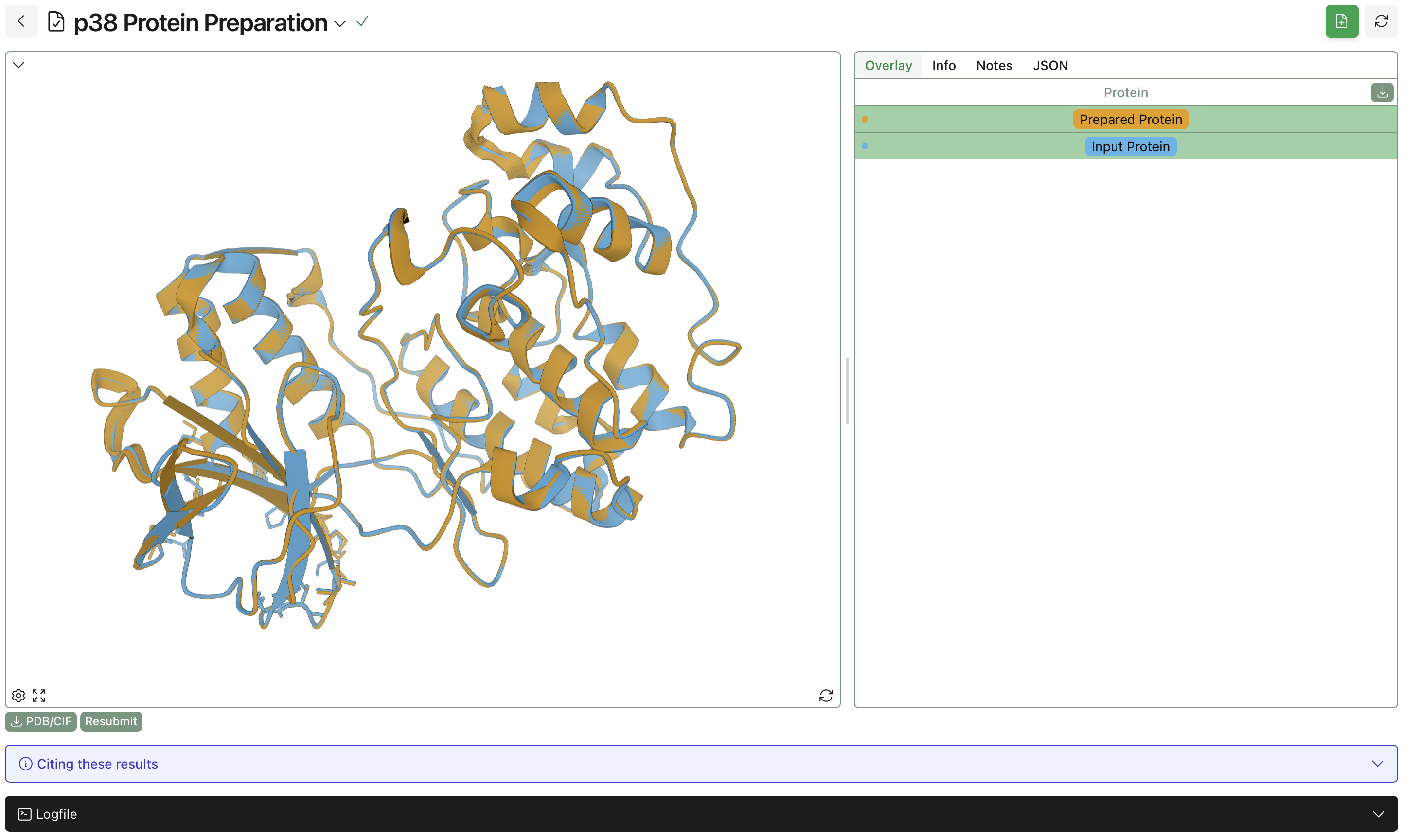
The first step is to load our desired protein, either from the PDB or, as in this case, from a local file. If the structure is not yet simulation-ready, our protein-preparation workflow is a great way to make sure the protein is ready for downstream modeling. We may also want to organize our campaign in a project and with folders, but this is optional. By default, submitted workflows will land in the root folder of your default project.

from pathlib import Path

import rowan

data_dir = Path(__file__).parent / "data"

rowan.project_uuid = rowan.get_project("p38 RBFE Python Demo", create=True).uuid
folder = rowan.get_folder("p38 RBFE")

protein = rowan.upload_protein(
    "p38", data_dir / "p38_structure.pdb", project_uuid=rowan.project_uuid
)
preparation_workflow = rowan.submit_protein_preparation_workflow(
    protein=protein,
    folder=folder,
    name="Prepare p38",
)
print(f"View: https://labs.rowansci.com/public/protein-preparation/{preparation_workflow.uuid}")

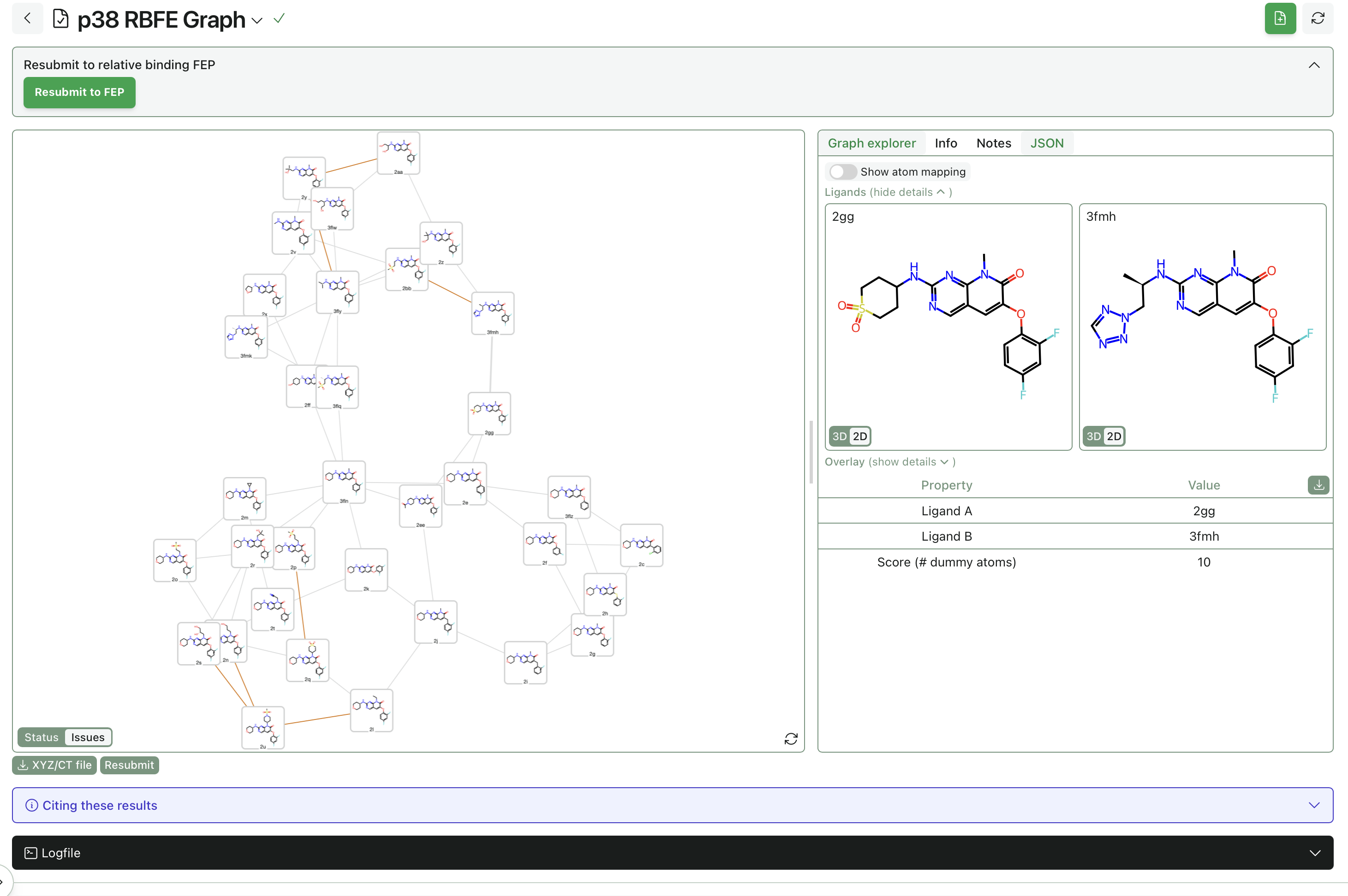
We also need to choose an analogue series and construct a perturbation graph using the RBFE graph workflow. To submit the graph workflow, we'll load an SDF file with ligands posed in the same coordinate space as the protein. Since our example is from the JACS benchmark set, we're starting with a set of posed ligands, but later in this tutorial we will demonstrate how to create this graph with only one bound reference ligand and a set of analogue SMILES.

preparation = preparation_workflow.result()
prepared_protein_uuid = preparation.prepared_protein_uuid

ligands = rowan.load_named_ligands(data_dir / "p38_ligands.sdf")
print(f"Loaded {len(ligands)} ligands: {', '.join(ligands)}")

graph_workflow = rowan.submit_relative_binding_free_energy_graph_workflow(
    ligands=ligands,
    folder=folder,
    name="p38 RBFE Graph",
)
print(
    "View: https://labs.rowansci.com/public/rbfe-graph/"
    f"{graph_workflow.uuid}"
)
graph = graph_workflow.result()
print(f"Built {len(graph.edges)} edges over {len(graph.ligands)} ligands")

Once we've prepared our protein and created an RBFE graph, we can submit both to the RBFE workflow. In this case, we'll first submit the workflow as a draft in order to retrieve a runtime estimate, as RBFE runs can span multiple hours if many perturbations are modeled. Instead of polling until the workflow completes, we recommend enabling an email alert or using a webhook.

fep = rowan.submit_relative_binding_free_energy_perturbation_workflow(
    graph_result=graph,
    protein=prepared_protein_uuid,
    tmd_settings="recommended",
    folder=folder,
    name="p38 RBFE",
    is_draft=True,
)

dispatch = fep.dispatch_info()
print(f"Estimated runtime: {dispatch.estimated_runtime_minutes} minutes")
print(f"Compute hardware: {dispatch.compute_hardware}")

fep.submit_draft()
fep.update(email_when_complete=True)
print(f"View: https://labs.rowansci.com/public/relative-binding-free-energy-perturbation/{fep.uuid}")
print(f"FINISHED_RBFE_UUID = {fep.uuid!r}")

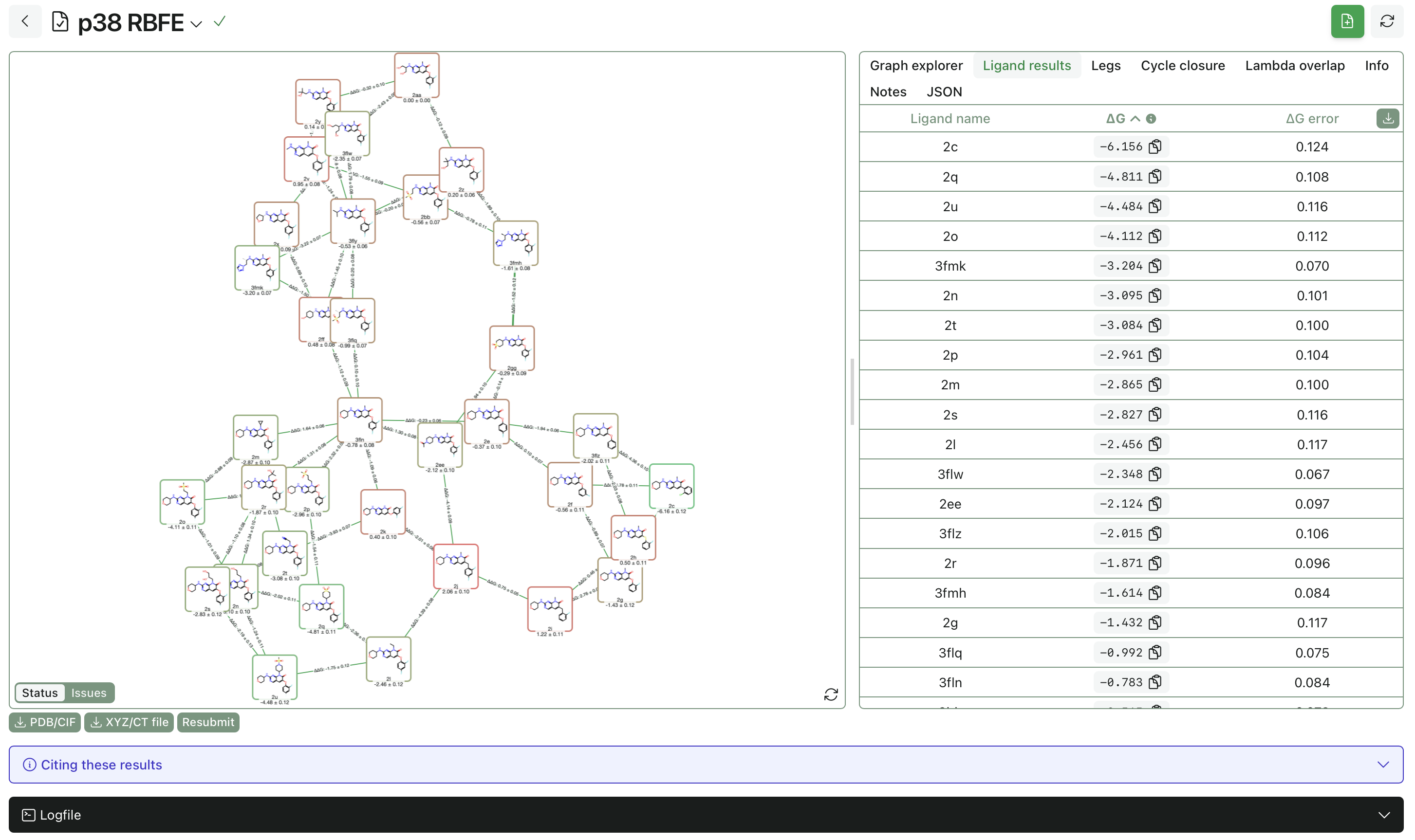
We split this code into snippets for explanation purposes, but this entire section can be executed as a single Python file.

Result Analysis

Once our RBFE workflow is finished, we can view its results directly in memory or download ΔGs as a CSV file to decide which analogues to simulate next.

import rowan

FINISHED_RBFE_UUID = "paste-the-uuid-printed-by-initial-run"

finished = rowan.retrieve_workflow(FINISHED_RBFE_UUID).result()
ranked_dgs = sorted(finished.ligand_dg_results.items(), key=lambda item: item[1].dg)

for name, prediction in ranked_dgs:
    print(f"{name}: ΔG = {prediction.dg:.2f} +/- {prediction.dg_err:.2f} kcal/mol")

print(f"Wrote {finished.write_ligand_results_csv('p38_rbfe_results.csv')}")

The RBFE result object also contains cycle-closure error, the complex-leg lambda-state overlap matrix, and per-edge ΔΔGs, all of which can be inspected to determine the quality of simulation results.

Iterative Design

After the initial RBFE simulation is complete and the new analogues are selected, the iterative design loop may begin. In a real campaign, these intermediate ligand generations could come from a medicinal chemist, an optimization model, or an agentic design workflow as discussed by Ishaan in our post on binder optimization with LLMs. To pose new compounds, we'll start by creating a dictionary with analogue names and SMILES (analogues chosen for this example are for demonstration purposes only) and retrieving the previously finished RBFE workflow.

import rowan

FINISHED_RBFE_UUID = "paste-the-uuid-printed-by-initial-run"

NEW_LIGANDS = {
    "new-1": "Cn1c(=O)c(Oc2ccc(Cl)cc2F)cc2cnc(NC3CCOCC3)nc21",
    "new-2": "Cn1c(=O)c(Oc2ccc(C)cc2F)cc2cnc(NC3CCOCC3)nc21",
    "new-3": "Cn1c(=O)c(Oc2ccc(F)cc2Cl)cc2cnc(NC3CCOCC3)nc21",
    "new-4": "Cn1c(=O)c(Oc2ccc(F)cc2F)cc2cnc(NC3CCOC3)nc21",
    "new-5": "Cn1c(=O)c(Oc2ccc(F)cc2F)cc2cnc(NC3CCCCC3)nc21",
    "new-6": "CCn1c(=O)c(Oc2ccc(Cl)cc2F)cc2cnc(NC3CCOCC3)nc21",
    "new-7": "N#CCn1c(=O)c(Oc2ccc(F)cc2F)cc2cnc(NC3CCS(=O)(=O)CC3)nc21",
    "new-8": "Cn1c(=O)c(Oc2ccc(OC)cc2F)cc2cnc(NC3CCOCC3)nc21",
    "new-9": "CC(C)n1c(=O)c(Oc2ccc(F)cc2F)cc2cnc(NC3CCOCC3)nc21",
    "new-10": "Cn1c(=O)c(Oc2ccc(C#N)cc2F)cc2cnc(NC3CCOCC3)nc21",
}

rowan.project_uuid = rowan.get_project("p38 RBFE Python Demo", create=True).uuid
folder = rowan.get_folder("p38 RBFE")

finished = rowan.retrieve_workflow(FINISHED_RBFE_UUID).result()

Next, we'll find bound poses for the new ligands using the analogue-docking workflow. This workflow uses one reference ligand to dock new ligands in the same pocket aligned along their maximum common substructure. We use the protein and a ligand directly from the completed RBFE workflow so that downstream simulations will be consistent with previous results.

dock_workflow = rowan.submit_analogue_docking_workflow(
    analogues=list(NEW_LIGANDS.values()),
    analogue_names=list(NEW_LIGANDS.keys()),
    initial_molecule=next(iter(finished.ligands.values())),
    protein=finished.protein,
    num_conformers_per_analogue=100,
    folder=folder,
    name="p38 Analogue Dock",
)
print(f"View: https://labs.rowansci.com/public/analogue-docking/{dock_workflow.uuid}")
dock = dock_workflow.result()

posed = {pose.name: pose for pose in dock.best_poses.values()}
print(f"Docked {len(posed)}/{len(NEW_LIGANDS)} new ligands")

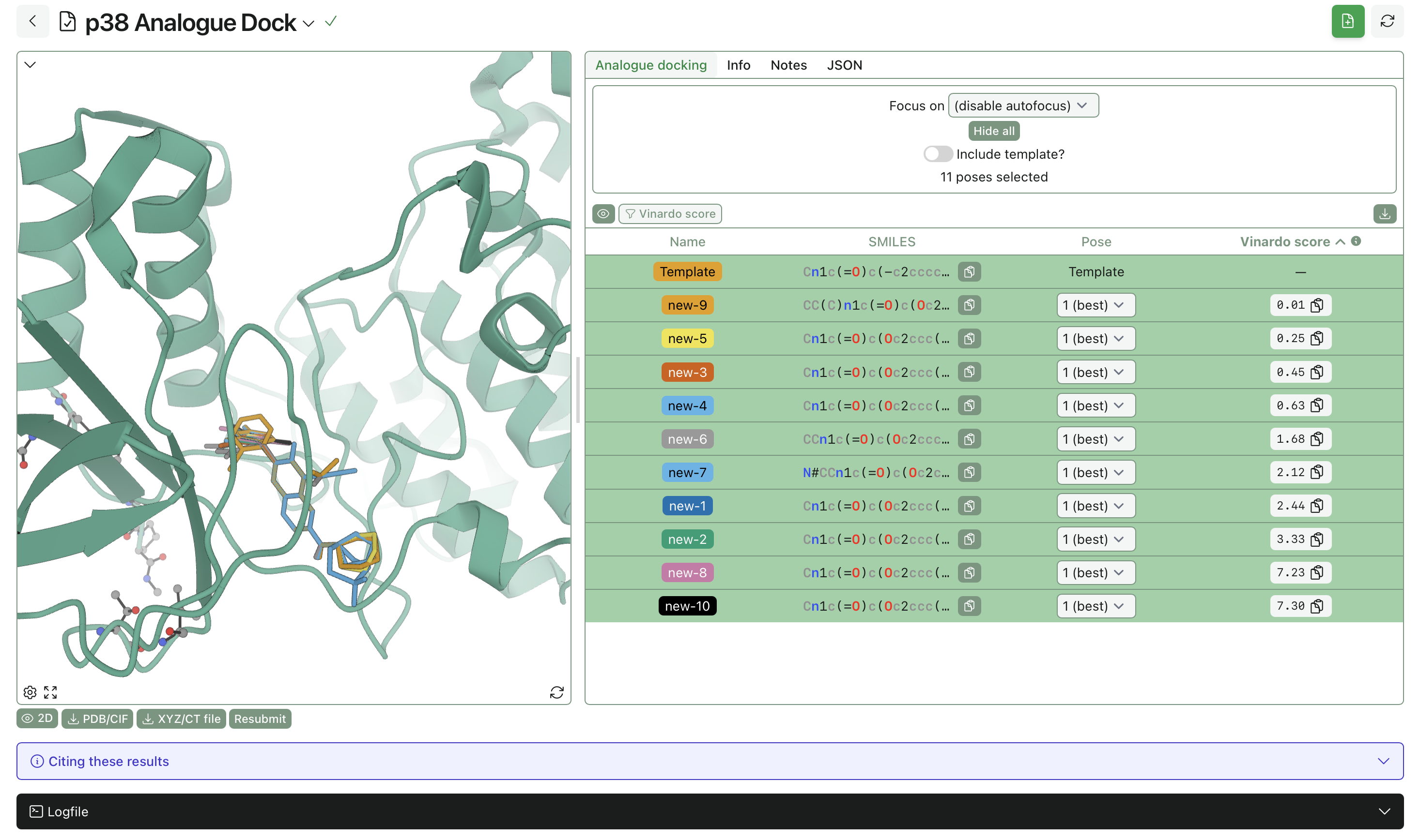
Once analogue docking is complete, we can extend the completed perturbation graph with the newly posed analogues. To do so, we'll pass the finished ligands along with the new analogues to the ligands field and pass the completed RBFE graph to the seed_graph field.

graph_workflow = rowan.submit_relative_binding_free_energy_graph_workflow(
    ligands={**finished.ligands, **posed},
    seed_graph=finished.graph,
    folder=folder,
    name="p38 with Analogues Graph",
)
print(
    "View: https://labs.rowansci.com/public/rbfe-graph/"
    f"{graph_workflow.uuid}"
)
graph = graph_workflow.result()

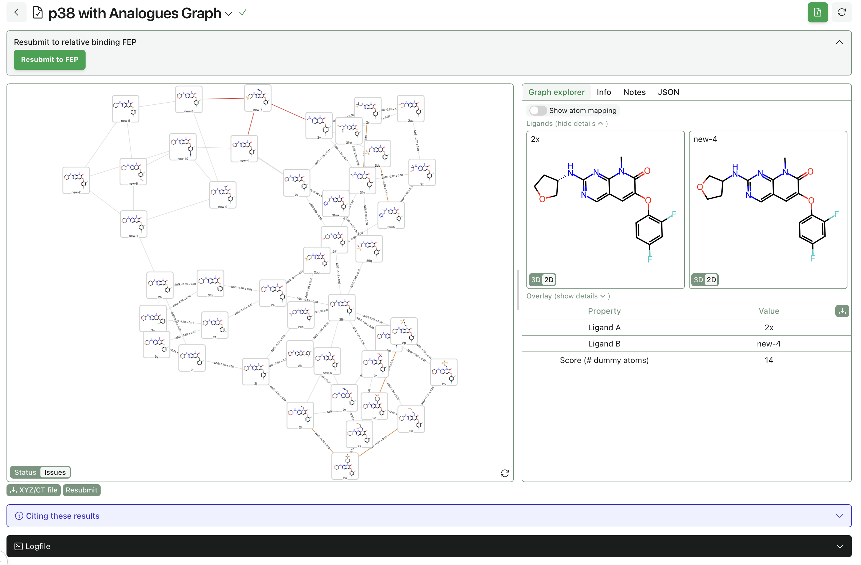
The resulting graph will have the new ligands and their perturbations along with the old ligands and their ΔΔG results. Legs resubmitted from a previous graph will not be rerun unless their results are cleared, so we can extend the graph without computing redundant simulations. We will pass this extended graph into an RBFE workflow along with the protein and settings from the previous RBFE run to simulate the new ligands and recompute the ΔGs for the entire graph.

fep = rowan.submit_relative_binding_free_energy_perturbation_workflow(
    graph_result=graph,
    protein=finished.protein,
    folder=folder,
    name="p38 with Analogues RBFE",
    is_draft=True,
    **finished.settings.model_dump(mode="json"),
)
dispatch = fep.dispatch_info()
print(f"Estimated runtime: {dispatch.estimated_runtime_minutes} minutes")
print(f"Compute hardware: {dispatch.compute_hardware}")

fep.submit_draft()
fep.update(email_when_complete=True)
print(f"View: https://labs.rowansci.com/public/relative-binding-free-energy-perturbation/{fep.uuid}")

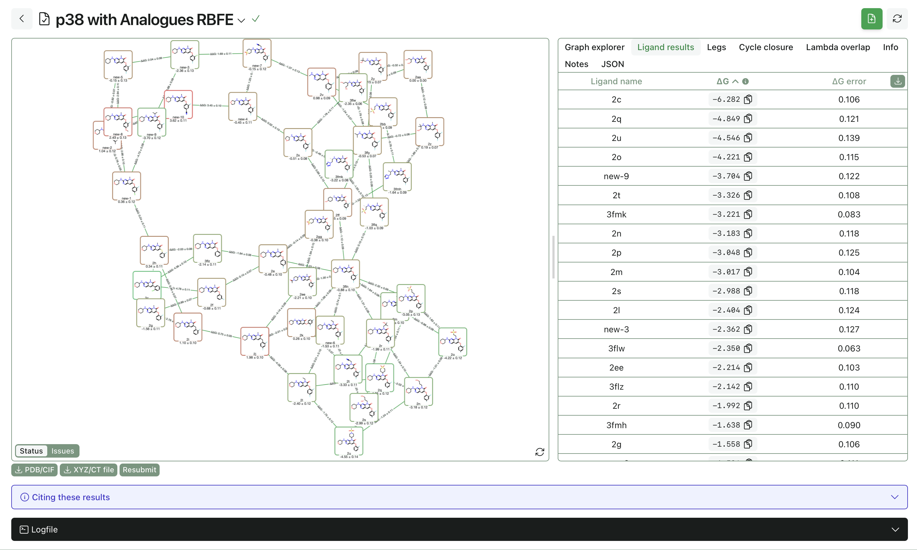
This simulation could also run for a number of hours depending on the system and the number of new analogues, so runtime estimation and asynchronous execution with completion notification is prudent.

All workflows submitted through the Rowan Python SDK can be viewed using Rowan's web platform as well, and all the workflows run in this tutorial can be found here. If you're interested in running programmatic FEP or agent-driven campaigns, we'd love to hear from you! You can reach us at contact@rowansci.com.