Improving Rowan's Performance on the OpenBind EV-A71 Release
by Corin Wagen · May 20, 2026
Last week, we posted our day-one results from the OpenBind data release; we selected a 76-compound subset, used analogue docking to generate poses from a random template structure, and ran Rowan's RBFE workflow against these poses to predict relative free energy values. (The input structures are available on GitHub.)
Our initial results were mixed. We successfully confirmed the sanity of our end-to-end pipeline: over 50% of our selected poses were within 1 Å of the crystallographic pose, and RBFE calculations starting from both the crystallographic and docked poses were within 1 kcal/mol MAE of the experimental values (ruling out any catastrophic failure scenarios). On the other hand, the results were predictively useless, with essentially no ability to rank-order binders.
An external observer might reasonably ask: why put such bad results on your blog? Doesn't this make your software look terrible? We share these results because we think it will be helpful to our customers. While we'd prefer Rowan's FEP to work perfectly out of the box every single time, this unfortunately doesn't happen in real life, and it's common to find cases where protocol tuning is needed to get useful FEP results—transparently documenting this process should be useful to external observers.
Here's what we wrote in the original post:
We expect that further protocol tuning or FEP improvements will be able to produce improved results; we haven't done any project-specific parameter tuning here and report these results simply as a zero-shot baseline about what's possible out of the box with FEP.
It's entirely possible that trivial modifications to our protocol will lead to improved performance. We've worked on this project for fewer than 24 hours, and report these data with the hope that others will do the same and push the field forward. Benchmarks drive scientific innovation, and tough and diverse benchmarks like OpenBind are exactly what's needed to push the free-energy field towards increased real-world predictive accuracy.
In this post, we'll share how we achieved useful FEP performance on a subset of our data: what worked, what didn't work, and what we plan to investigate moving forward.
Simple Protocol Changes
We first tried simply adjusting the RBFE protocol along a few dimensions, keeping the same 76 docked poses (pKD range 5.03–7.94) and the same 138-edge RBFE graph:
- We switched from NAGL charges (our default) to the typical AM1BCC charge-assignment method. AM1BCC is slower, particularly for large molecules, since a separate set of semiempirical calculations has to be run for each input molecule, but there are sometimes meaningful differences between the two charge methods. In this case, we didn't see any big differences (compare rows 1 & 2), but we used AM1BCC for the remaining rows because that's generally accepted and has fewer potential confounding pathologies.
- We tried simply running each window for longer. By default, TMD runs 2 ns simulations per window; bumping this up to 4 ns didn't produce significant improvement in our hands (compare rows 2 & 3).
- We tried decreasing the number of global steps. By default, 390 of every 400 steps are "local" MD steps which rely only on a 12 Å radius about the ligand; we've sometimes seen that lowering this to 350 is helpful. This seemed to meaningfully reduce error and slightly improved ranking accuracy, although the changes were a bit too small to interpret (compare rows 2 & 4).
- Since reducing the number of local steps seemed to help, we decided to go all the way and run RBFE without any local MD steps (our "rigorous" default settings). This matches how non-TMD programs operate, and here it led to substantial improvements: a Pearson correlation value of 0.3, for instance (compare rows 2, 4, and 5).
| run | main change | RMSE (kcal/mol) | MAE (kcal/mol) | Pearson | Spearman | Kendall |
|---|---|---|---|---|---|---|
| 1 | (baseline) | 1.064 | 0.810 | 0.071 | 0.065 | 0.039 |
| 2 | AM1BCC charges | 1.108 | 0.863 | -0.071 | -0.104 | -0.073 |
| 3 | AM1BCC + 4 ns windows | 1.071 | 0.839 | -0.011 | -0.015 | -0.009 |
| 4 | AM1BCC + 350 local steps | 0.987 | 0.791 | 0.115 | 0.032 | 0.029 |
| 5 | AM1BCC + no local steps | 0.913 | 0.701 | 0.304 | 0.273 | 0.187 |
Pyrrolidine Subset Analysis
At this point, it seemed unlikely that further protocol changes were going to magically give us great performance on the full 76-compound set. We looked through the compounds to see if some smaller subset of the data was well-described at the "rigorous" level of theory. which would let us zoom in and better understand where these errors were coming from.
We identified a 32-compound subset of compounds which all shared a common pyrrolidine scaffold and which seemed to perform better at the rigorous level of theory (Spearman rho of 0.67, Kendall tau of 0.51). To double-check our poses, we also redocked all compounds to x7026b (shown below), a relatively unsubstituted member of the series.
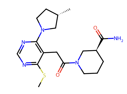
Compound x7026b, a simple member of the pyrrolidine series.
The resulting poses overlaid very well, with only the substituents on the pyrrolidine really varying.
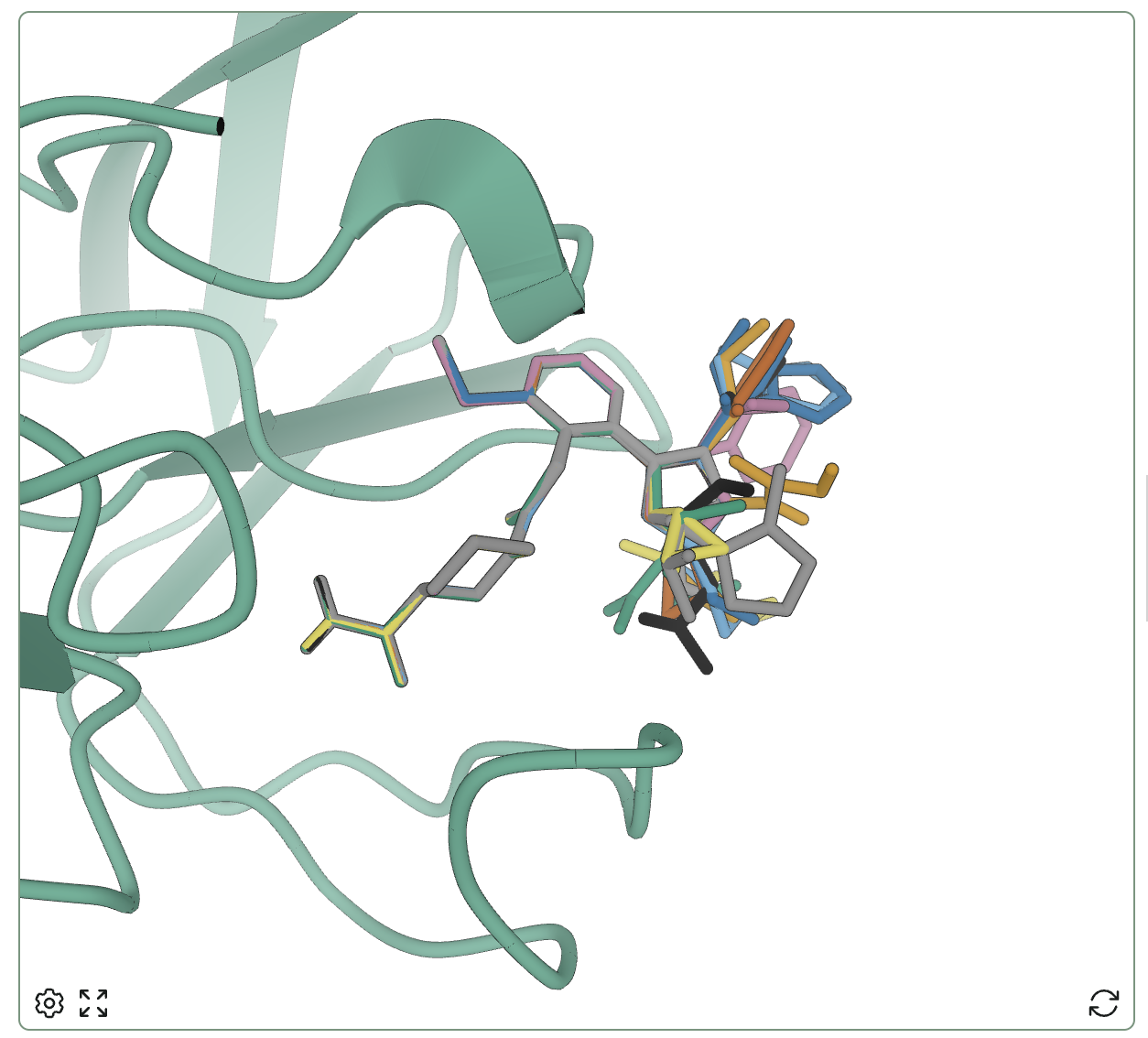
The selected pose for all 32 pyrrolidine binders, overlaid.
We ran eight more RBFE runs focusing on the 32 pyrrolidine structures.
| run | pose source | settings | RMSE (kcal/mol) | MAE (kcal/mol) | Pearson | Spearman | Kendall | Runtime (h) |
|---|---|---|---|---|---|---|---|---|
| 6 | docked | default/NAGL | 1.119 | 0.870 | 0.281 | 0.228 | 0.157 | 4.38 |
| 7 | docked | default/AM1-BCC | 1.032 | 0.817 | 0.415 | 0.350 | 0.270 | 4.92 |
| 8 | docked | 350 local (2 nm) /AM1-BCC | 1.067 | 0.860 | 0.344 | 0.274 | 0.206 | 8.93 |
| 9 | docked | rigorous/AM1-BCC | 1.062 | 0.838 | 0.348 | 0.361 | 0.278 | 18.72 |
| 10 | redocked | rigorous/AM1-BCC | 1.204 | 0.930 | 0.212 | 0.087 | 0.071 | 18.39 |
| 11 | crystal | default/NAGL | 1.268 | 0.981 | -0.006 | -0.010 | -0.012 | 4.63 |
| 12 | crystal | default/AM1-BCC | 1.197 | 0.946 | 0.087 | 0.038 | 0.046 | 5.21 |
| 13 | crystal | rigorous/AM1-BCC | 1.026 | 0.746 | 0.426 | 0.464 | 0.399 | 20.06 |
Overall, the best run was the rigorous run starting from crystallographic poses (run 13), although other protocols achieved non-zero accuracy (better than in the full 76-compound set above). Here's the scatter plot for the best run—not amazing, but there's now some predictive power.
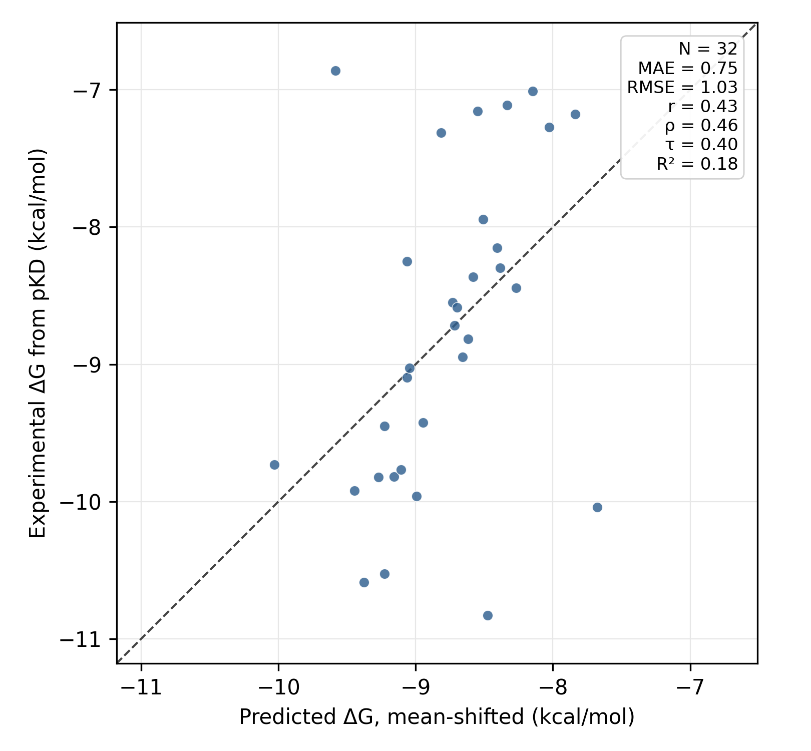
Results from RBFE Run #13.
Pose Error
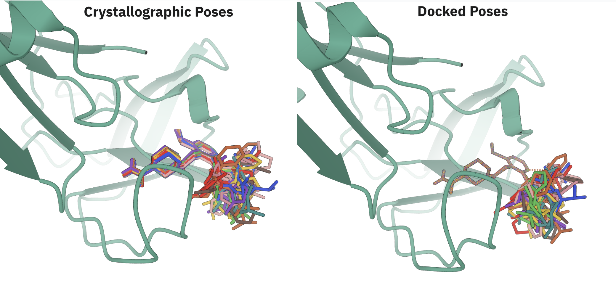
The above data shows that the crystallographic poses were consistently better than the docked poses (and different docking runs gave very different results). We wanted to understand this more: since prospective FEP usage can rarely benefit from extensive crystallographic support, getting a robust pose-preparation pipeline is critical.
To start, we used Rowan's strain workflow to check the strain of both sets of poses (the full set, not just the pyrrolidines). Here's a visual summary of the strain of the docked poses—even without doing any particularly advanced analysis, you can see that there's a substantial number of compounds with strain above 5 kcal/mol, and even a few with strain over 10 kcal/mol.
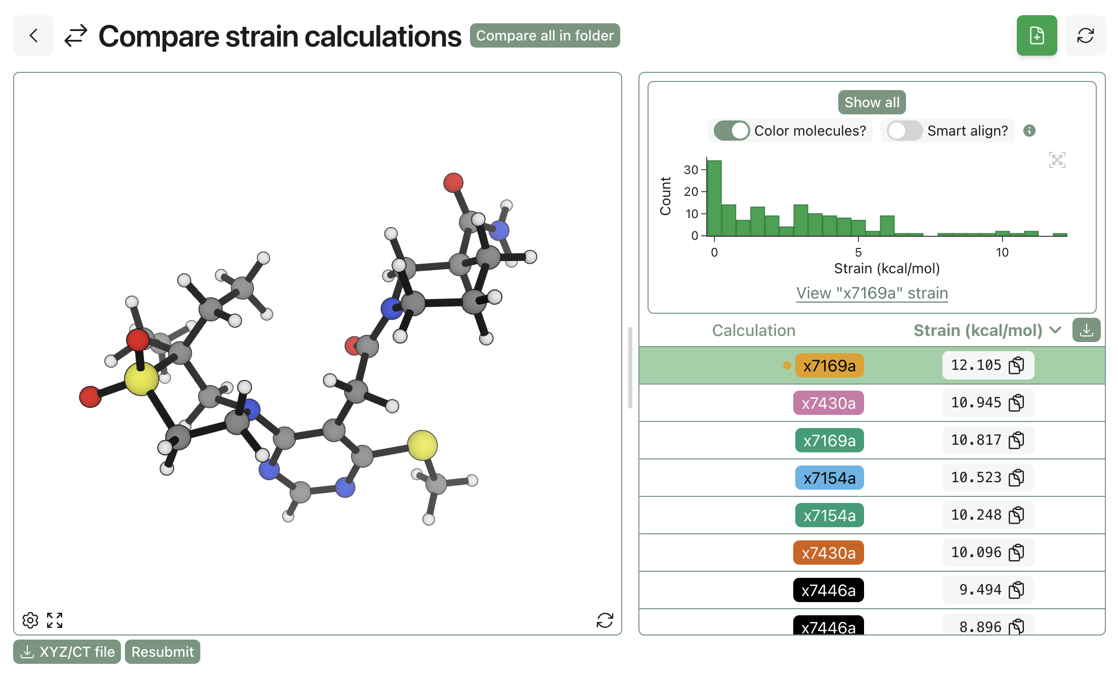
Strain for docked poses.
In contrast, only a single crystallographic pose has a strain above 5 kcal/mol:
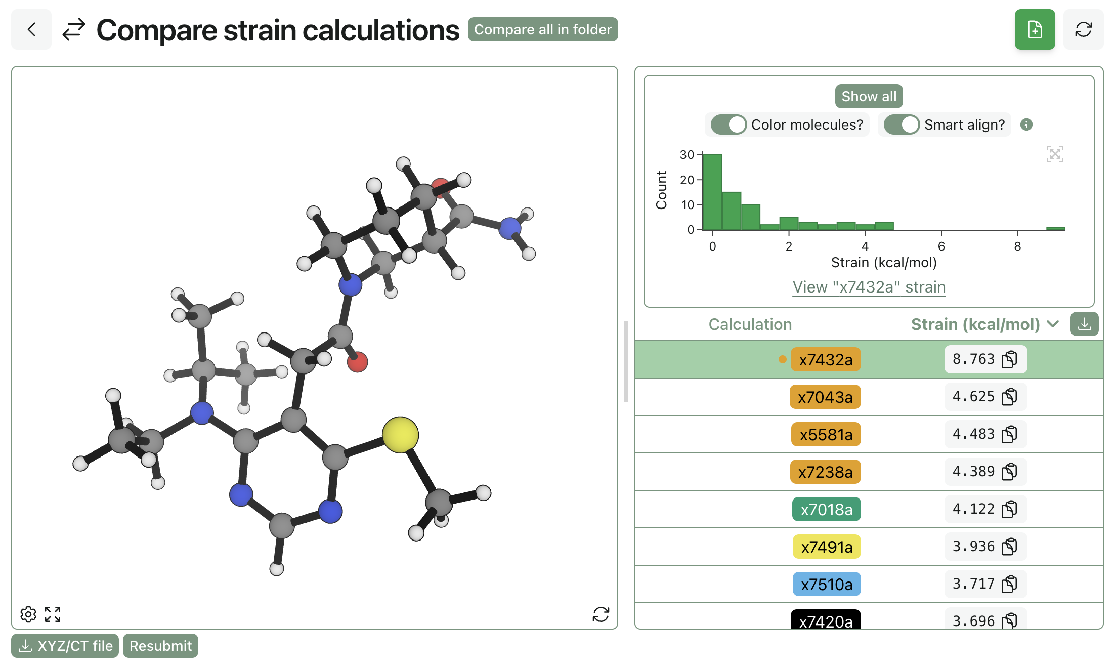
Strain for crystallographic poses.
This suggests that the crystallographic poses don't just happen to be better for FEP. Instead, they're better because they're systematically lower in energy and generally more physical. The bad news is that our analogue-docking workflow isn't working perfectly, but the good news is that the quality of our FEP runs will improve if we can improve the pose-preparation pipeline.
We zoomed in on a few cases with particularly large changes. The predicted binding affinity of compound x7161a changed a lot between docked and crystallographic poss (0.8 kcal/mol or so, depending on protocol), which could be ascribed to a change in the conformation of the pendant methoxymethyl group:
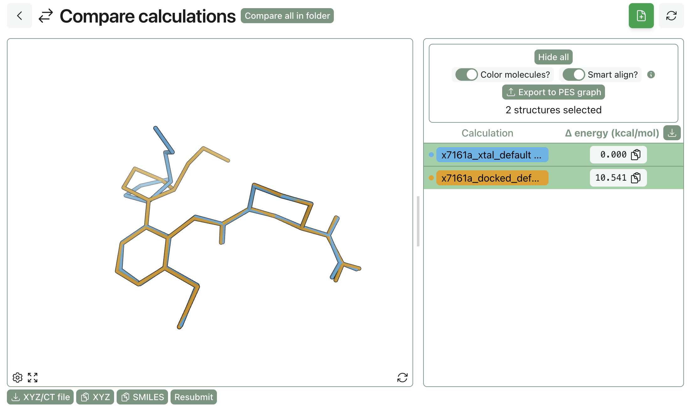
Comparison of the docked and crystallographic poses for x7161a.
Compound x7247a had the largest change between docked and crystallographic poses (3.66 Å RMSD), essentially flipping the pyrrolidine and moving a pyrazole substituent from one face to the other:
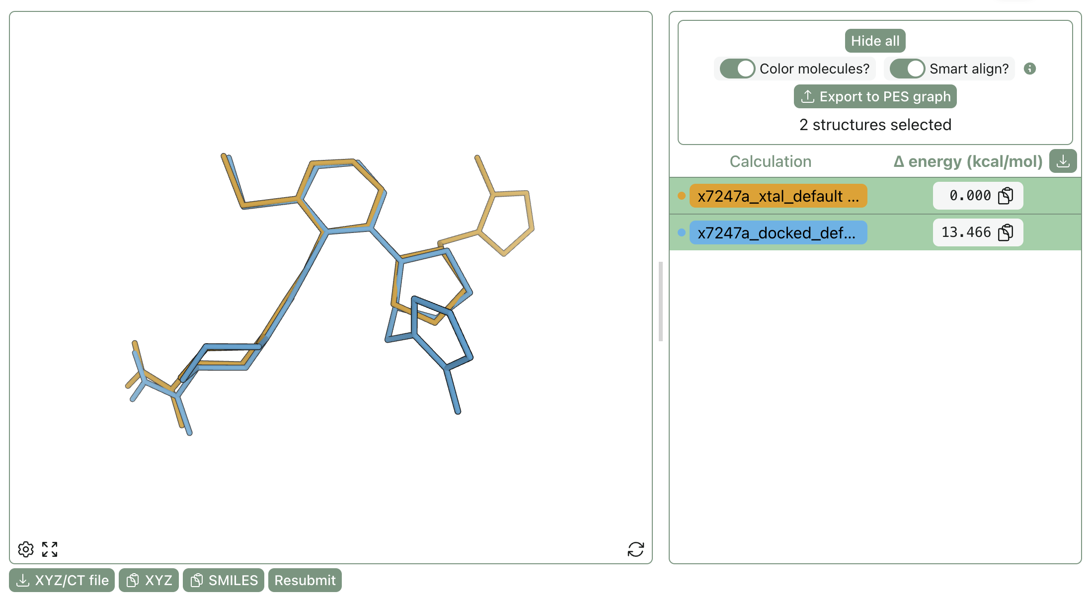
Comparison of the docked and crystallographic poses for x7247a.
Overall, the data support the idea that pose preparation is a significant source of error for these results, although even crystallographic poses don't lead to stellar RBFE performance. It's worth noting that the big issue here isn't pose generation, it's selection—we're able to generate a large ensemble of poses, we just don't yet have a good way to tell which one to use for FEP calculations.
Economic Impact
Stepping back—is this worth it in real drug-discovery programs? The best FEP run ranked compounds with an accuracy of 0.464 (Spearman ) and cost about $550 in GPU time, or about $17 per compound. The best accuracy obtained without crystallographic poses was 0.361 (Spearman ), which more closely mimics how FEP would be used in the real world.
Quantifying economic value is tough, but the extremes are obvious—an FEP protocol that ranks compounds with is clearly useless and a waste of money, while a protocol that ranks things perfectly () would be very useful.
To try and model the cases in the middle, we built a toy simulation model that takes unknown "true" rankings and generates imperfect computational rankings with the same Spearman correlation observed in our RBFE benchmark. (Implementation details below for the curious.) We then ask—if we synthesize the top 10 compounds from the imperfect ranking, how many of the true top-10 compounds will actually be in that set? (We'll call this enrichment factor .)
Here's what the model predicts. At , because we're just picking randomly, while at we're getting all 10. At the more realistic value of , we predict that . We're getting some enrichment but most "good virtual compounds" still aren't that good.
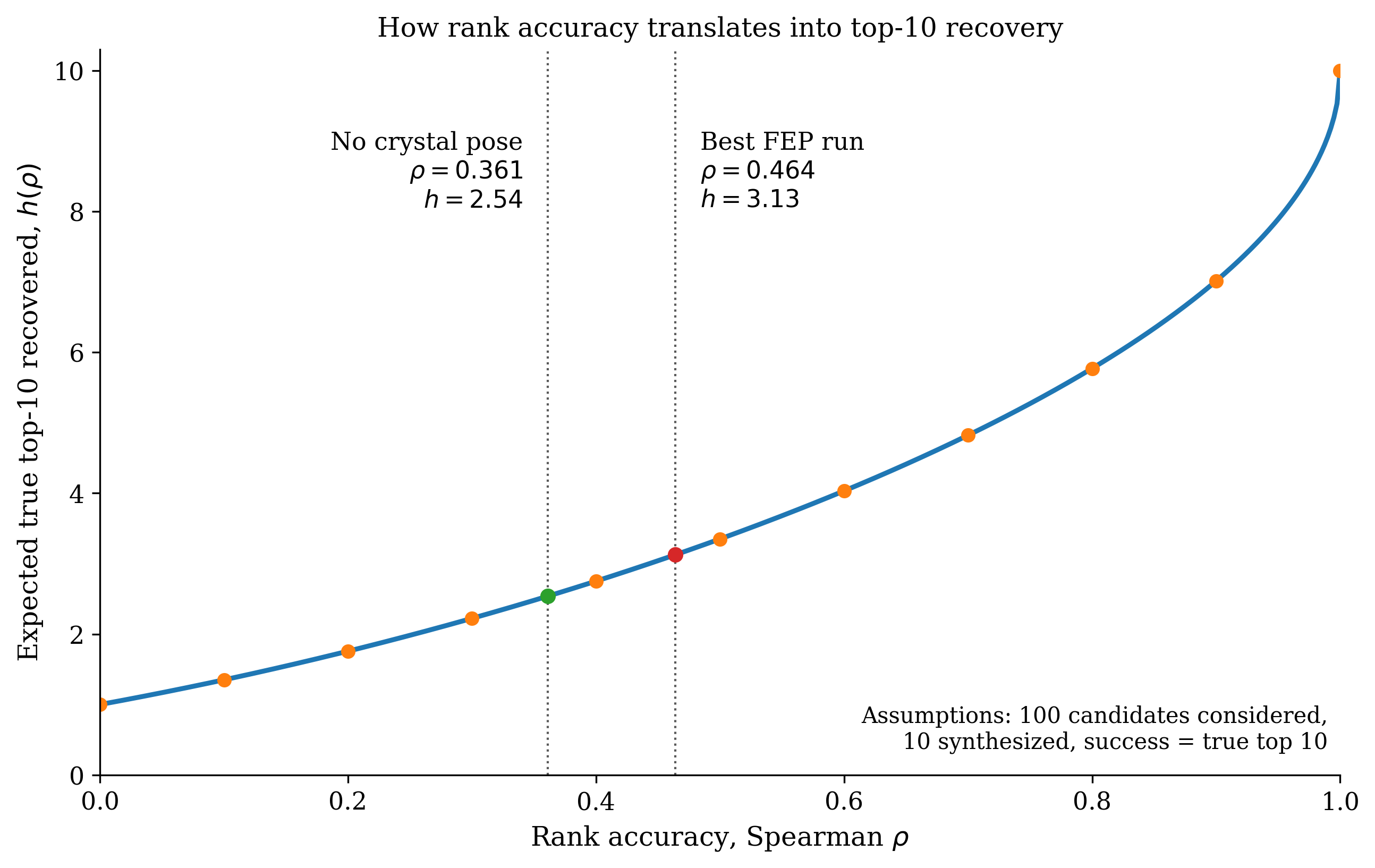
Dependence of on .
Now to try and figure out if this is worth it. If is the number of good compounds selected using RBFE and is the number of good compounds selected without RBFE, then the net dollar value per cycle is:
where is the all-in synthesis and assay cost per wet-lab compound, is the number of virtual compounds screened, is the cost of running an RBFE calculation, and is the number of compounds actually synthesized and tested.
I'll choose some simple numbers here:
- varies a ton based on targets, compounds, CROs and so on — I'll put $2,000 here.
- To keep things simple, we'll keep modeling the scenario where we're modeling 100 compounds and synthesizing 10 ( and ).
- , as stated above, is $17 per run. We'll round up to $20 to make sure we're being sufficiently pessimistic.
All together, versus random selection, we find that FEP creates about $28,700 of net value per 100-compound design cycle, or roughly $2,900 per compound actually synthesized in the 10-compound experimental tranche.
(The maximum value in this model is $178,000, corresponding to essentially getting 90 compounds or $180,000 worth of screening for only $2000 of in silico screening.)
Of course, this example is a bit rigged, and "drug discovery without FEP" does not usually imply "pick compounds at random." Medicinal chemists, docking, property filters, and lower-cost predictive models already provide some prioritization signal. The key question is how good that existing triage process is. In this toy model, the FEP protocol remains value-positive at the assumptions above as long as the baseline process recovers fewer than about 2.31 of the true top-10 compounds per cycle, corresponding to a rank correlation of roughly . Against a weaker baseline, FEP is worth about $6,900 per cycle; against a baseline, it is still slightly positive at about $800 per cycle.
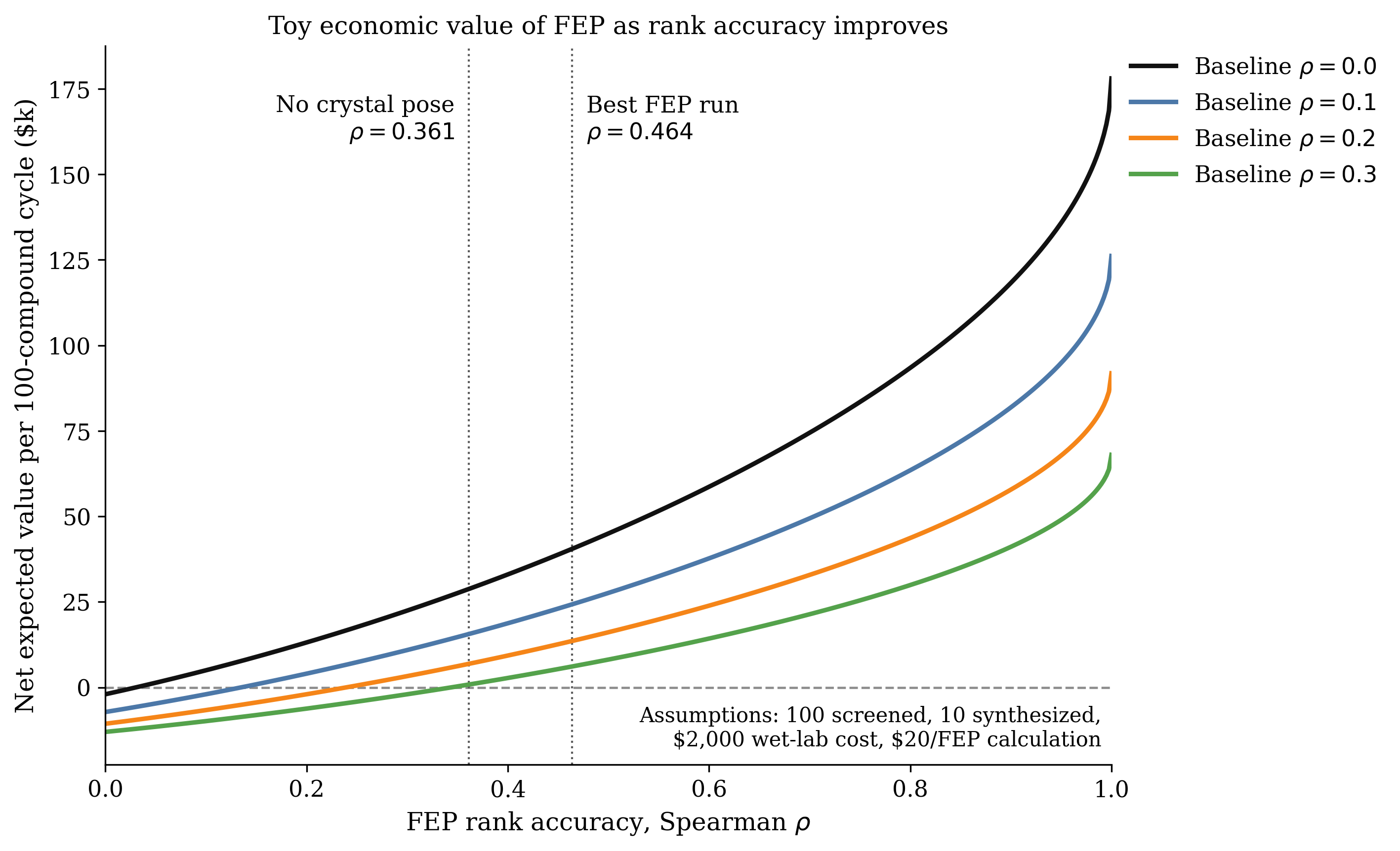
The expected value of FEP based on .
The takeaway is not that FEP is always worth running—every company, program, and target are different, and nobody should use the above simplistic model as "proof" that FEP will or won't work for them. Rather, this model demonstrates that even moderately accurate FEP can be economically valuable when wet-lab slots are expensive and the existing prioritization stack is meaningfully weaker than the FEP model. At $20 per candidate, the computational cost is small enough that even modest improvements in experimental hit recovery can be worth it. (In fact, in the naïve model, per-compound RBFE costs of up to $307 are still expected-value positive.)
Conclusions
First, we hope that this post illustrates what running FEP in the real world can be like—it's more complicated than the oft-cited standard benchmarks might make it appear! If your initial FEP runs don't give the accuracy that you're hoping for, there are a lot of knobs to tune to try and recover useful performance (even apart from any improvements that we make here at Rowan). Different poses, different simulation settings, and different subsets of compounds can all lead to major differences in the utility of RBFE.
Second, we hope that this post is encouraging. Even if your FEP run doesn't give perfect rank correlation, running RBFE at scale can still be quite useful—provided that the extra expense of the software license and the skills needed to run RBFE doesn't erase these gains. That's part of why we're committed to making Rowan's FEP offering as fast, cheap, and easy to use as possible… making FEP cheaper, faster, and better will let more scientists and companies benefit from increased predictive power.
Third, this exercise helps us decide what we're going to work on next at Rowan. We would like Rowan FEP to work as well as possible, and we're planning to address some of the issues that this OpenBind dataset has highlighted:
- We need to make our pose-selection logic more intelligent and more robust, potentially by integrating strain or single-point MM/GBSA calculations. (This dataset will let us test a variety of approaches, which is great.)
- We need to more robustly handle tricky transformations like those found in the larger initial set, potentially through adding artificial alchemical intermediates to break tricky transformations down into simpler ones.
- We hope to investigate refitting new forcefields for different areas of chemical space, which might help minimize errors arising from poor forcefield description of e.g. torsions.
- We need many more automatic checks for convergence, bad atom mapping, and simulation accuracy. We shouldn't have to figure out if simulations need to be run for longer simply by running longer and longer simulations in a loop…
- And we want to make everything faster and cheaper for our users.
If you're in early-stage drug discovery and you're interested in building or testing any of these features in conjunction with our team, please reach out! We love working alongside drug-discovery scientists to validate and stress-test new scientific functionality.
Appendix: Generating Realistic Imperfect Rankings
The model needs a way to generate an imperfect computational ranking with a specified Spearman rank correlation to the unknown "true" experimental ranking.
A convenient way to do this is:
- Generate a latent "true experimental score" for each compound.
- Generate a latent "computational score" that is correlated with .
- Rank compounds by to define the true experimental ordering, and by to define the computational ordering.
We assume the latent scores are jointly normal:
where controls how strongly the computational score tracks the true score.
Because our benchmark accuracy is reported as Spearman rank correlation rather than ordinary Pearson correlation, we choose so that the resulting rankings have the desired Spearman . For jointly normal variables, population Spearman correlation and latent Pearson correlation are related by , so we set .
Once those paired rankings are generated, the rest is simple:
- take the top 10 compounds in the computational ranking;
- ask how many are also in the true experimental top 10;
- repeat many times and average.
This gives the expected recovery value .
Thanks to GPT 5.5 for helping me work through the statistics here.