Benchmarking Membrane-Permeability Predictors
by Ari Wagen · Apr 28, 2026

Saint Paul Escapes from Damascus by Philip Galle after Maerten van Heemskerck
Three months ago we added two membrane-permeability predictors to Rowan: GNN-MTL, a neural network trained on AstraZeneca permeability data, and PyPermm, a physics-based permeability predictor. The obvious question is: where do these methods actually work?
To answer this question, we benchmarked both methods across four membrane permeability datasets spanning small molecules, cyclic peptides, and macrocycles—plus, as a challenge, a PROTAC oral bioavailability dataset.
Methods
GNN-MTL is a ChemProp model trained on internal AstraZeneca permeability data from Ohlsson et al. 2025. GNN-MTL was trained to predict apparent membrane permeability in the absorptive apical-to-basolateral direction in the presence of transporter inhibitors (Papp AB+).
PyPermm is a Python reimplementation of the physics-based PerMM method from Lomize and Pogozheva 2019. PyPermm calculates intrinsic membrane permeability in the absorptive apical-to-basolateral direction with no transports as well (P0 AB+). For PyPermm, 3D conformers were generated using RDKit's ETKDGv3 method followed by up to 200 steps of MMFF optimization. This conformer-generation procedure is likely too simplistic for highly flexible or conformationally complex molecules such as macrocycles and cyclic peptides, which may negatively affect PyPermm's performance on those datasets.
For comparison, we also evaluate two simple baseline descriptors: hydrogen-bond donor count (HBD) and quantitative estimate of druglikeness (QED). Because additional hydrogen-bond donors generally reduce passive membrane permeability, HBD count acts as a simple heuristic predictor of permeability.
Note: the experimental datasets aren't always perfectly aligned with the quantities predicted by either model. Many public datasets report apparent permeability without transporter inhibition, adjusted data from mixed assay conditions, or, to the best of our knowledge, don't clearly state exactly which permeability measure they're reporting. This isn't something we can totally control; we're noting it here, and readers should keep this in mind for this blog post and any other methods studying public ADME data.
Data cleaning
Taking some advice from this 2023 Pat Walters blog post, we applied several cleaning steps to reduce ambiguity in these benchmark sets:
- molecules with undefined stereochemistry or ambiguous E/Z geometry were removed,
- inconsistent duplicate measurements (>0.3 log units disagreement) were excluded, and
- all retained structures were validated with RDKit.
These filters were not applied to the PROTAC dataset.
Wang et al. Caco-2
The Caco-2 data from Wang et al. 2016 is perhaps the best-known permeability dataset, as a cleaned version of this dataset is included in the Therapeutic Data Commons as "Caco2_Wang." This means that it's in the training data of most public ML permeability methods; however, we can use this a somewhat external benchmark because the GNN-MTL model was trained only on data internal to AstraZeneca (though we can't certainly rule dataset leakage out).
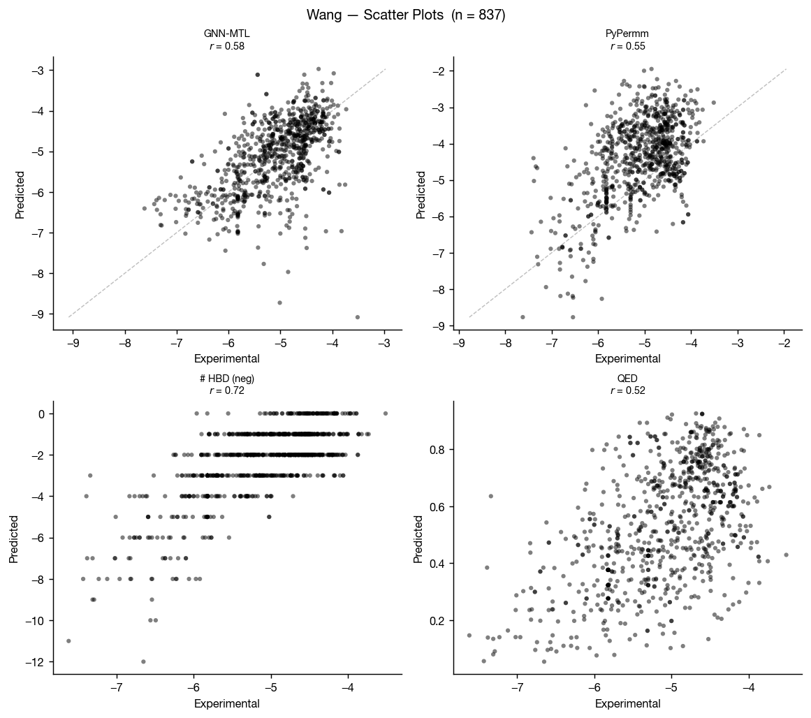
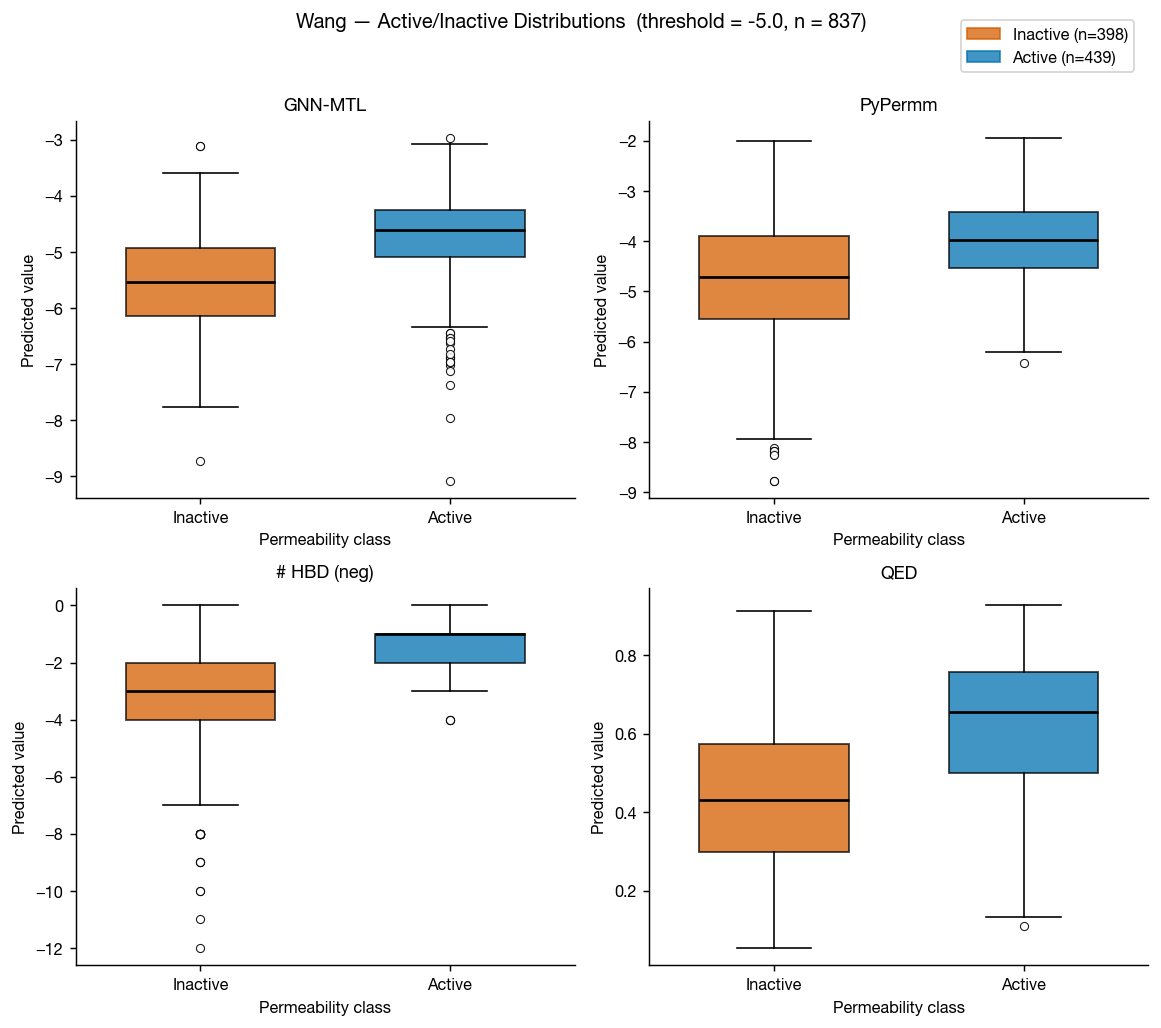
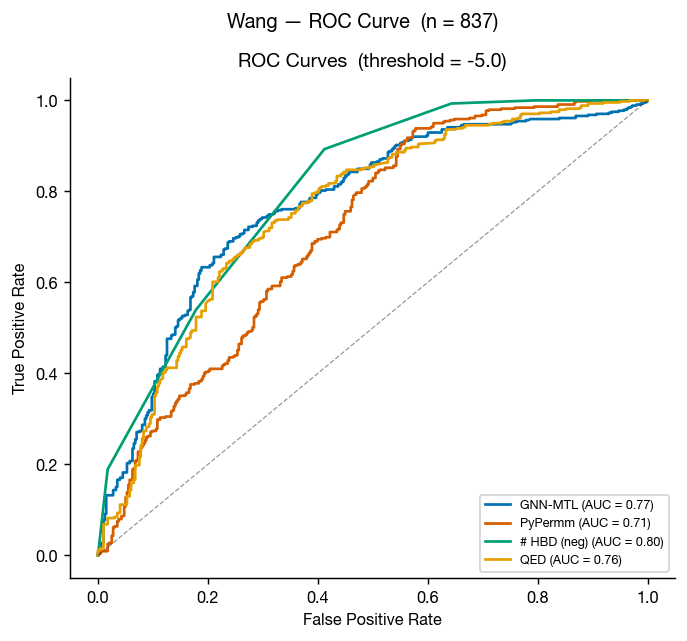
These results don't surprise: GNN-MTL (trained on small molecule data) edges PyPermm out, though both show fair ability to differentiate between compounds with low and high measured permeabilities.
Wang et al. additional Caco-2
Wang et al. 2016 also includes a compiled set of measured permeabilities of FDA approved small molecules. This a much smaller dataset, but it's another helpful test set for us here.
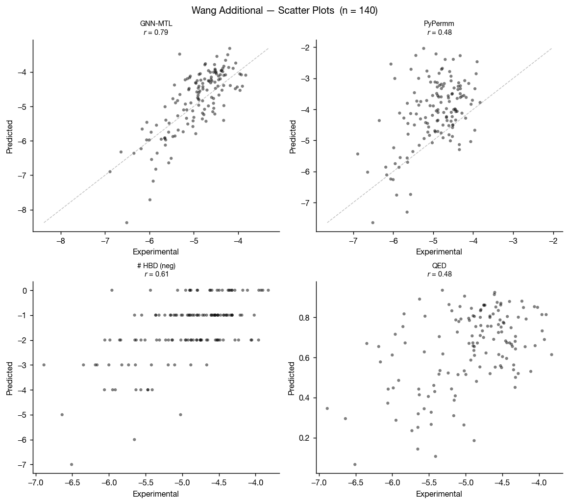
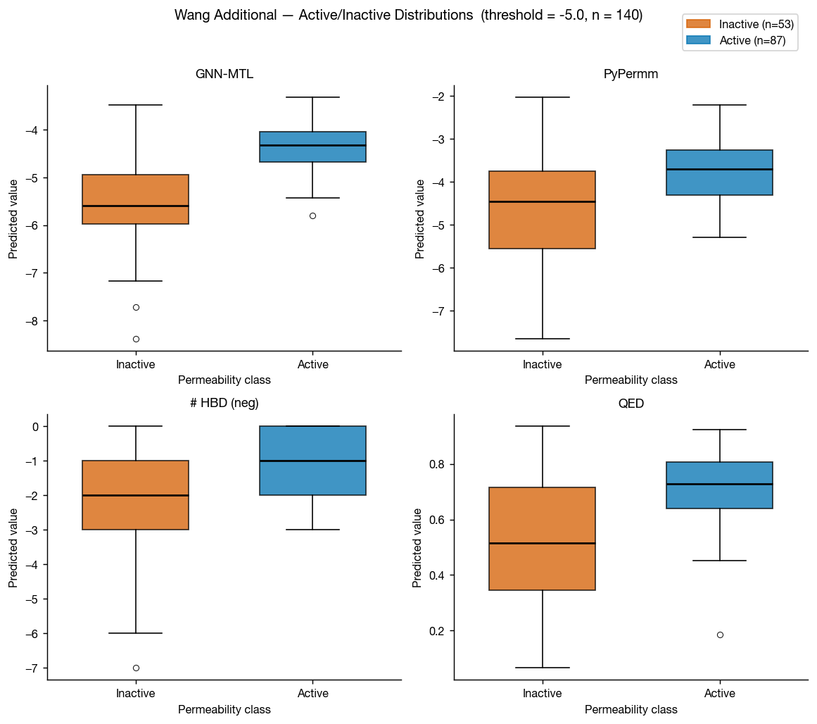
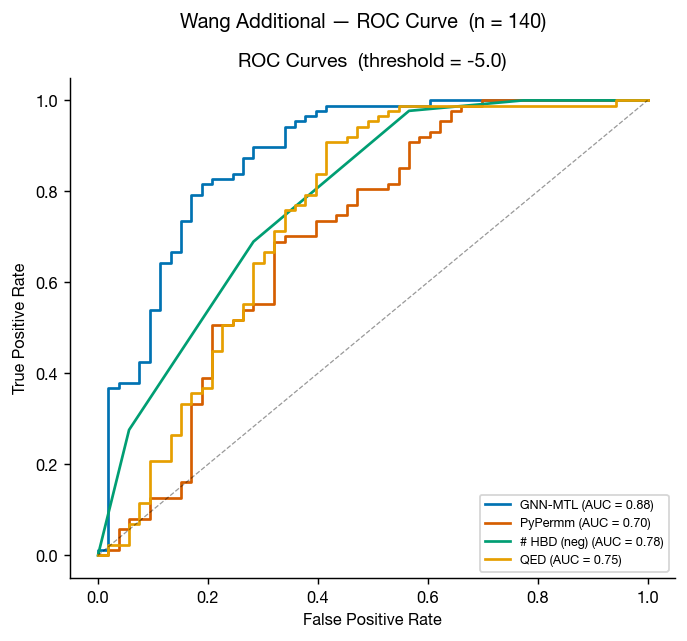
As in the primary Wang dataset, GNN-MTL performs better on conventional small molecules while both methods retain useful discriminatory power.
CycPeptMPDB
CycPeptMPDB is a database of cyclic peptides with measured membrane permeabilities, reported in Li et al. 2023 and available at cycpeptmpdb.com. We benchmarked our methods against the subset of this database with reported Caco-2 values.
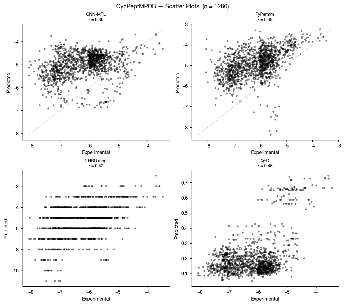
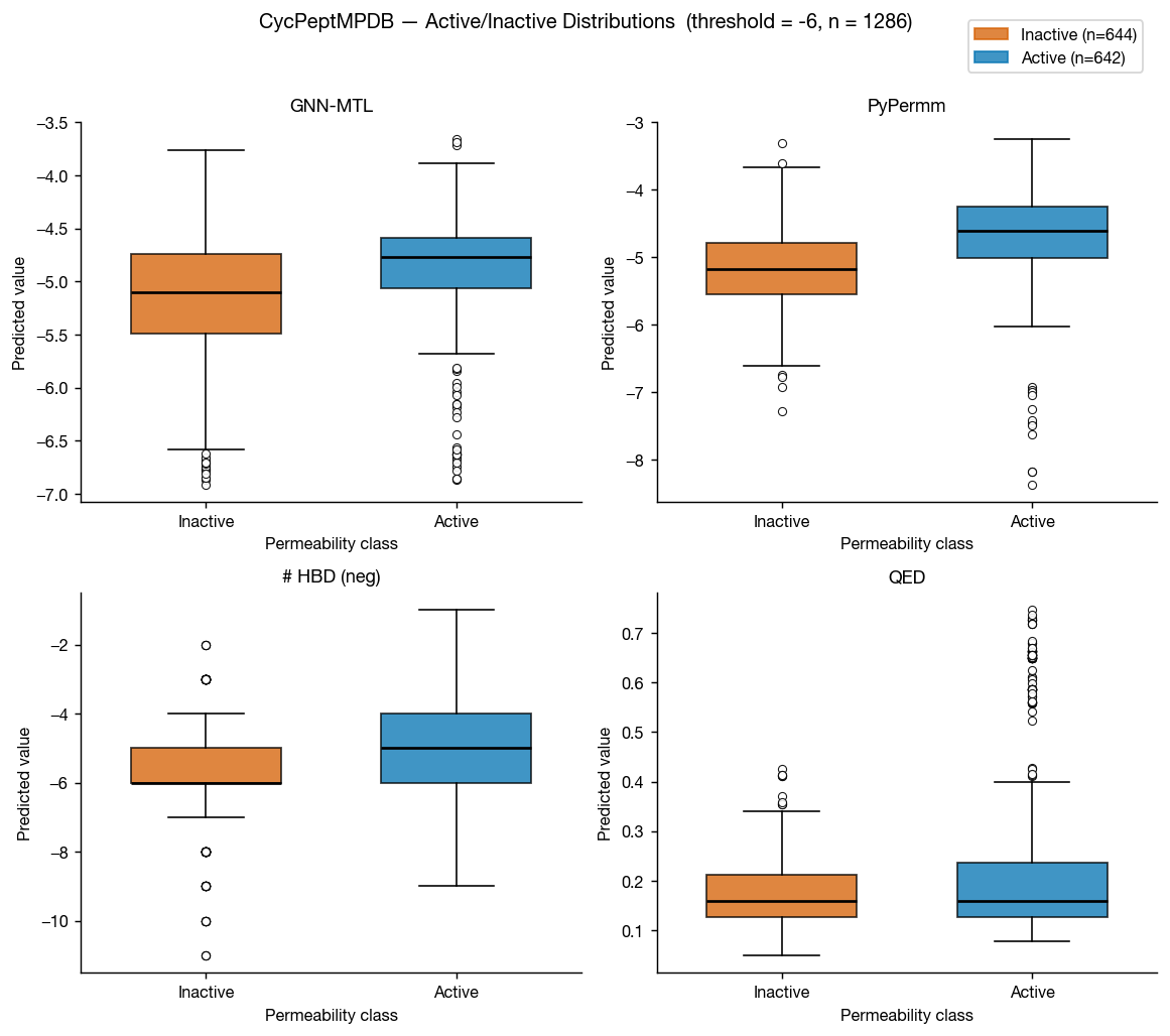
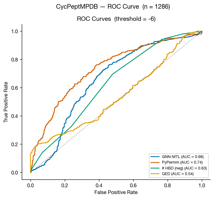
Again, the methods perform similarly, but as we move outside of traditional small-molecule space, it seems that PyPermm is taking a slight lead, showing better separation and higher AUC.
NPMMP-DB
The non-peptidic macrocycle membrane permeability database (NPMMP-DB) is a database of cyclic macrocycles with measured permeabilites, reported in Feng at al. 2025 and available at swemacrocycledb.com. We benchmarked our methods against the 119 compounds with reported Caco-2 Papp AB+ data.
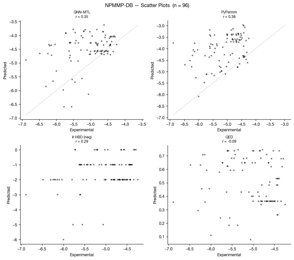
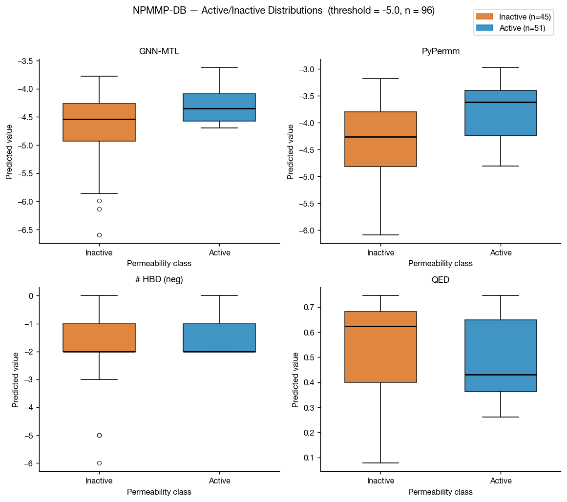
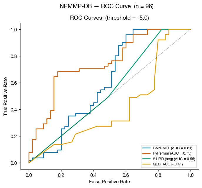
This benchmark is much smaller than the previous three, so the graphs tell a noisier story for these non-peptidic macrocycles. That said, the results suggest PyPermm could meaningfully exclude non-permeable compounds.
Apprato et al. PROTAC oral bioavailability
As a final challenge for these methods, we found a compiled dataset of 55 PROTACs with measured oral bioavailabilities in Apprato et al. 2024 via Baylon et al. 2025. Because membrane permeability is often thought to be a major driver of oral bioavailability for these large, flexible molecules, we expected compounds predicted to be more permeable to also show higher oral bioavailability. Instead, both permeability predictors failed almost completely. This may indicate that permeability alone is a poor model of oral bioavailability here, that these methods fail to capture PROTAC permeability, or both.
The BPILDD descriptor
The Baylon et al. paper introduces BPILDD, a modified version of the balanced permeability index (BPI) designed for ligand-directed degraders (LDDs): large, flexible molecules where oral bioavailability is often limited by poor permeability. The descriptor combines lipophilicity, molecular shape, polarity, and size:
where SMID is the smallest maximum intramolecular distance, PSA is polar surface area, and HAC is heavy atom count.
The authors first demonstrate the utility of BPILDD at separating highly absorbed compounds from poorly absorbed ones on an internal dataset of 129 cereblon-recruiting degraders. They argue that orally available degraders "successfully balance the trade-off between minimizing polarity and attaining a more elongated, rod-like shape."
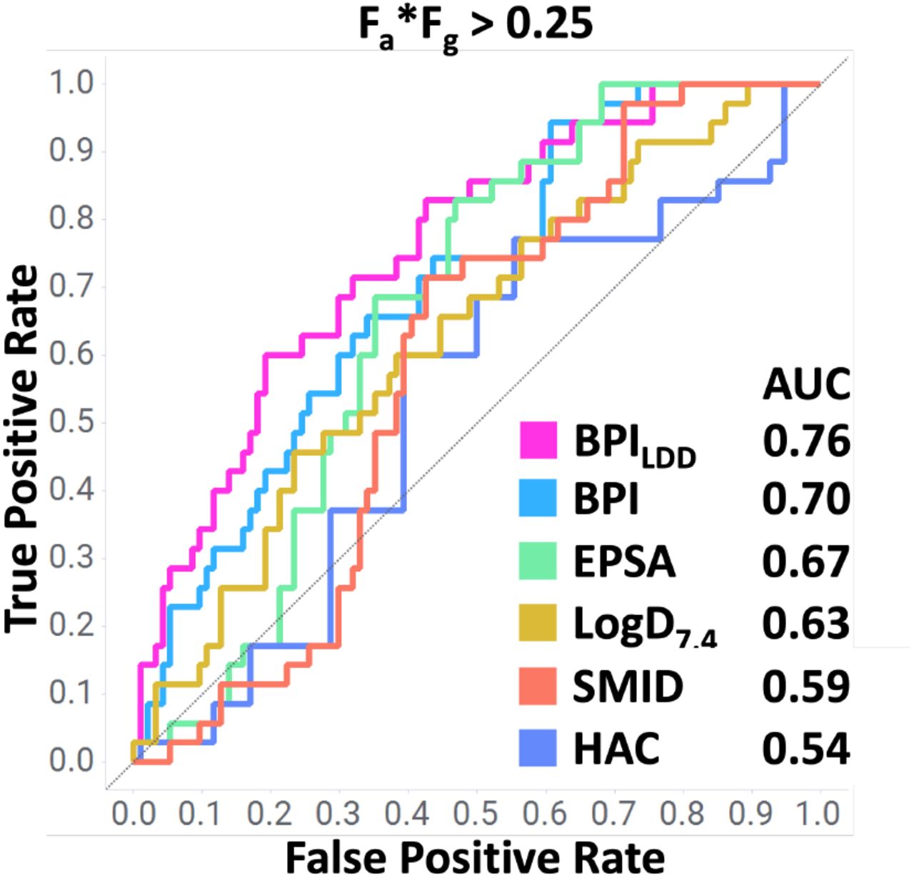
Figure 1 from Baylon et al. 2025.
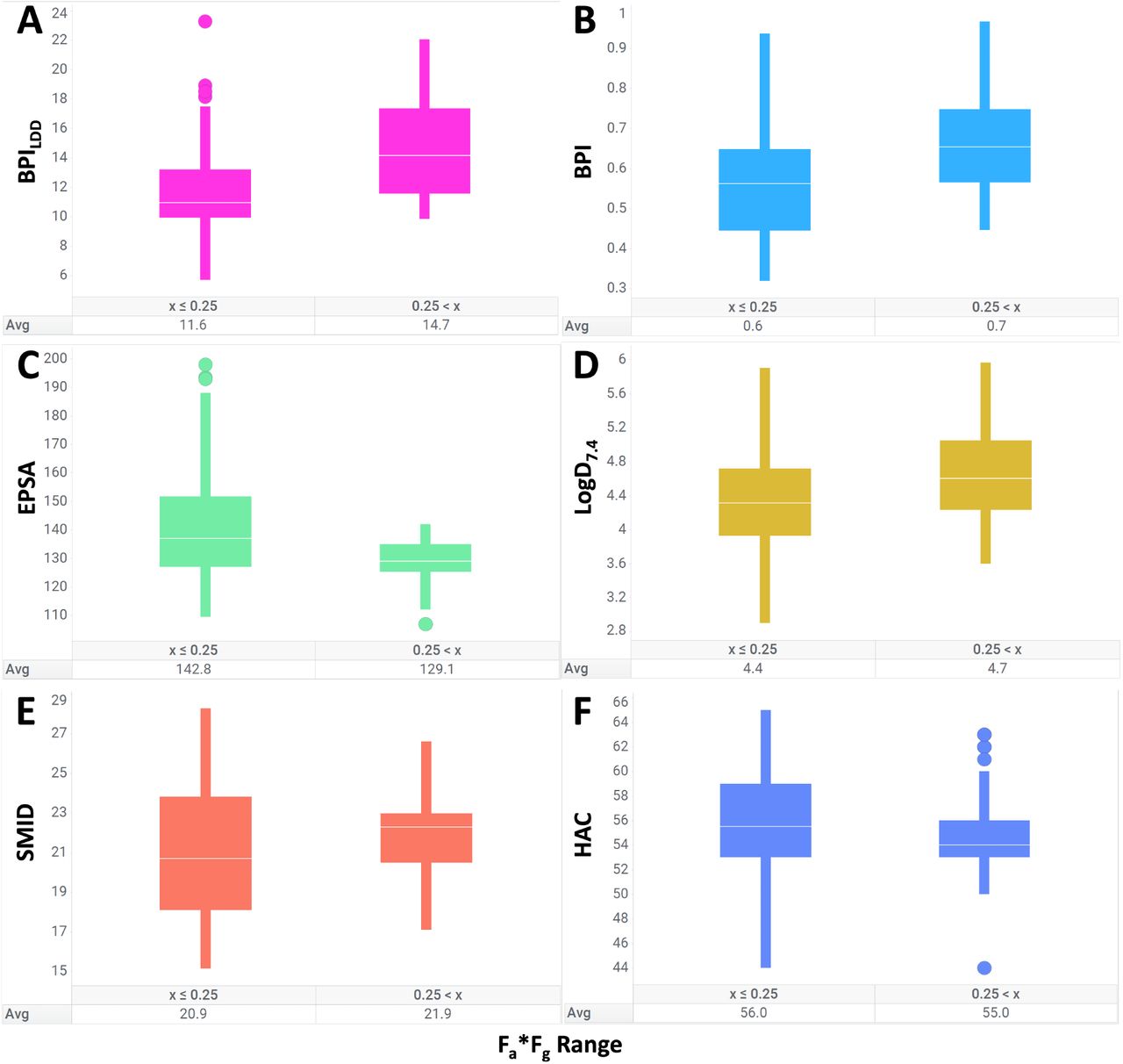
Figure 2 from Baylon et al. 2025.
Results on the Apprato et al. dataset
The data in this dataset were compiled from different sources, and 46 of the 55 SMILES representations in the dataset contain unassigned stereocenters (raising a number of concerns about the consistency and quality of the data).
When calculating the BPILDD descriptor for this dataset, Baylon et al. substituted cLogP and TPSA instead of experimental logD and EPSA values when calculating the BPILDD descriptor. The authors note that this reduced performance relative to their internal dataset.
In addition to Rowan's membrane-permeability prediction methods, we also ran our ADMET and solubility prediction workflows on this 55-compound set. The results are underwhelming:
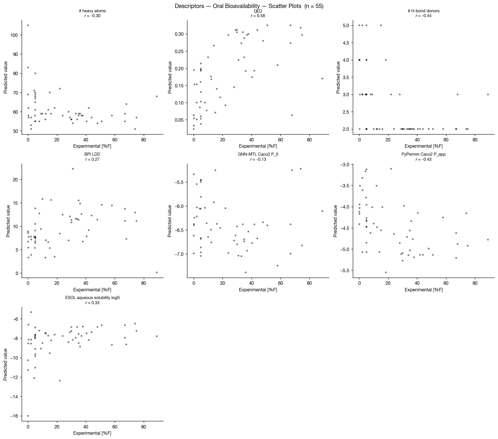
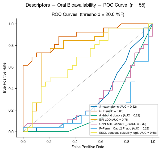
Although ESOL-predicted aqueous solubility shows some correlation with oral bioavailability, neither GNN-MTL nor PyPermm appears to capture a meaningful signal in this dataset.
In both methods, predicted permeability is actually anti-correlated with bioavailability, producing an apparent inverse relationship between predicted permeability and observed oral bioavailability. This is unlikely to reflect a causal permeability–bioavailability relationship.
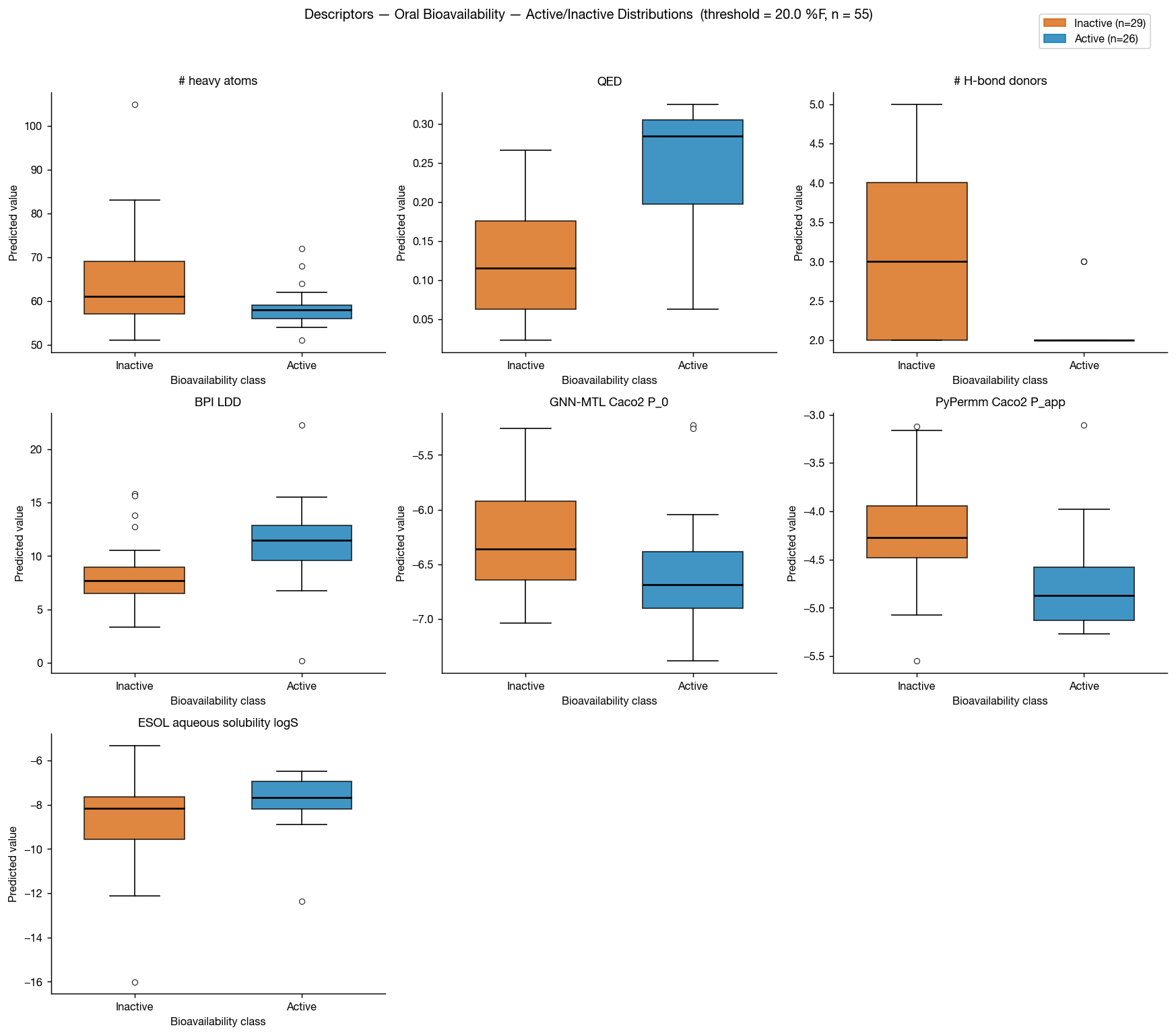
The predicted values themselves show little separation across the dataset: PyPermm values are almost entirely in the "good" permeability range while GNN-MTL's predictions are all in the "poor" regime, with little dynamic range between compounds. Together, this suggests that these permeability methods are not meaningfully distinguishing compounds in a way that explains the observed bioavailability trends.
Another surprising result is that QED and number of hydrogen-bond donors both as as excellent discriminators on this dataset, with AUCs of 0.88 and 0.22 (0.78 if inverted) respectively.
The authors themselves point out that simple baselines perform unusually well on this public set:
Unsurprisingly, the performance of BPILDD is degraded by the lack of experimental data (AUC = 0.73), likely due to underperforming contribution from cLogP. It is also unsurprising that HAC and TPSA perform similarly to the BPI metrics for enriching molecules with high oral bioavailability, and this is because this data set is comprised of multiple chemical series, including VHL and CRBN targeting LDD, with a large range of sizes and polarities.
That caveat is important. Public datasets assembled from many unrelated chemical series can contain strong structural biases. In these cases, simple descriptors may appear far more predictive than they would in a real lead optimization campaign, where compounds are usually much more chemically similar.
Summary of results
In practice, permeability predictors are often used as binary filters ("likely permeable" vs "unlikely permeable"). That introduces two separate thresholding problems:
- choosing a threshold for the experimental dataset labels (what counts as "permeable"), and
- choosing a threshold for the model predictions themselves.
For these datasets, we used a threshold of log(Papp in cm/s) = −5 to define permeability. One exception was CycPeptMPDB, where a −5 cutoff produced an extremely imbalanced dataset (positive rate 0.07), so the threshold was relaxed to −6.
| Dataset | N | Positive rate | Threshold | GNN-MTL (AUC) | PyPermm (AUC) | # HBD (AUC) | QED (AUC) |
|---|---|---|---|---|---|---|---|
| Wang | 837 | 0.52 | −5 | 0.77 | 0.71 | 0.80 | 0.76 |
| Wang Additional | 104 | 0.62 | −5 | 0.88 | 0.70 | 0.78 | 0.75 |
| CycPeptMPDB | 1286 | 0.50 | −6* | 0.66 | 0.74 | 0.63 | 0.54 |
| NPMMP-DB | 96 | 0.53 | −5 | 0.61 | 0.75 | 0.55 | 0.41 |
| PROTAC oral bioavailability %F | 55 | 0.47 | 20% | 0.30 | 0.22 | 0.78 | 0.88 |
Using these dataset-defined thresholds, the AUC results suggest a consistent pattern: GNN-MTL performs better on traditional small molecules, while the physics-based PyPermm model extrapolates more effectively to larger macrocyclic systems.
However, AUC alone can overstate practical utility because real-world use requires converting continuous predictions into binary decisions. A second threshold must therefore be chosen for the predictor outputs themselves.
The simplest approach is to ignore slight assay and unit mismatches between the experimental measurements and predictor outputs (e.g. experimental Papp AB vs predicted P0 AB+) and use the same numerical threshold for both (for example, classifying predictions above −5 as permeable when the dataset itself used a −5 cutoff). This works reasonably well for the small-molecule datasets, but performs poorly for CycPeptMPDB.
| Dataset | Winner | GNN-MTL Balanced Acc. | PyPermm Balanced Acc. | GNN-MTL Threshold | PyPermm Threshold | GNN-MTL vs PyPermm (McNemar) | GNN-MTL balanced vs. random | PyPermm balanced vs. random | Either beats majority? |
|---|---|---|---|---|---|---|---|---|---|
| Wang | GNN-MTL | 0.722 | 0.673 | −5 | −5 | Not significant (p=0.079) | Significant (p=0.0001) | Significant (p=0.0001) | True |
| Wang Additional | GNN-MTL | 0.805 | 0.656 | −5 | −5 | Significant (p=0.035) | Significant (p=0.0001) | Significant (p=0.0002) | True |
| CycPeptMPDB | PyPermm | 0.519 | 0.521 | −6 | −6 | Not significant (p=0.828) | Not significant (p=0.095) | Not significant (p=0.071) | False |
| NPMMP-DB | GNN-MTL | 0.611 | 0.600 | −5 | −5 | Not significant (p=1.000) | Significant (p=0.014) | Significant (p=0.026) | True |
If predictor thresholds are instead optimized independently for each model (using Youden's J statistic, which selects the threshold that maximizes the balance between sensitivity and specificity), performance improves substantially for the macrocycle datasets (CycPeptMPDB and NPMMP-DB).
However, this also highlights a practical issue: selecting optimal thresholds a priori is difficult. The shifts between the dataset-defined thresholds and the empirically optimized predictor thresholds suggest that calibration may differ substantially across chemical domains and model classes.
| Dataset | Winner | GNN-MTL Balanced Acc. | PyPermm Balanced Acc. | GNN-MTL Threshold | PyPermm Threshold | GNN-MTL vs PyPermm (McNemar) | GNN-MTL balanced vs. random | PyPermm balanced vs. random | Either beats majority? |
|---|---|---|---|---|---|---|---|---|---|
| Wang | GNN-MTL | 0.726 | 0.680 | −4.901 | −5.038 | Not significant (p=0.150) | Significant (p=0.0001) | Significant (p=0.0001) | True |
| Wang Additional | GNN-MTL | 0.814 | 0.684 | −4.812 | −4.099 | Significant (p=0.015) | Significant (p=0.0001) | Significant (p=0.0001) | True |
| CycPeptMPDB | PyPermm | 0.653 | 0.690 | −5.064 | −5.022 | Significant (p=0.034) | Significant (p=0.0001) | Significant (p=0.0001) | True |
| NPMMP-DB | PyPermm | 0.680 | 0.754 | −4.683 | −3.730 | Not significant (p=0.533) | Significant (p=0.0002) | Significant (p=0.0001) | True |
Takeaways
On the small-molecule datasets, the machine-learned GNN-MTL model outperformed the physics-based PyPermm method. But that advantage weakened—and in some cases reversed—as we moved into cyclic peptides and macrocycles. PyPermm generalized more effectively outside traditional drug-like chemical space, despite weaker performance on small molecules.
This highlights a broader lesson: strong performance on one chemical domain does not guarantee transferability to another. Models trained on conventional small molecules may struggle when applied to larger, more flexible compounds with very different conformational and physicochemical behavior.
The benchmarks also showed how important threshold calibration is in practice. Several datasets performed poorly when using fixed permeability cutoffs, but improved substantially after optimizing thresholds for the dataset at hand. A model with a reasonable ROC-AUC may still perform poorly as a real decision-making filter if its outputs are not calibrated appropriately for the target chemical space.
The PROTAC oral bioavailability benchmark reinforced another important point: oral bioavailability is not reducible to permeability alone. Neither permeability predictor captured a meaningful signal in this dataset, and both produced counterintuitive anti-correlations with observed bioavailability. Meanwhile, simple descriptors like hydrogen bond donor count and QED performed surprisingly well. This likely reflects a combination of dataset bias, mixed chemical series, and the fact that bioavailability depends on many interacting processes beyond passive membrane permeation.
Ultimately, there's no substitute for fine-tuned program-specific ADME modeling on your own project's internal data. Global methods like these can't achieve the same specificity as hand-crafted permeability predictors for a specific chemical series. When the requisite data for artisanal models is unavailable though—when a project is in its earliest stages, when the chemical space under exploration is extremely diverse, or when a new class of compounds is being considered—global methods like these can offer meaningful predictive accuracy right out of the box.
For a more in-depth review of permeability prediction methods, we recommend Storchmannová et al.'s recent paper "Meta-Analysis of Permeability Literature Data Shows Possibilities and Limitations of Popular Methods."
Try it yourself
If you want to try Rowan's membrane-permeability methods on your data, consider subscribing to Rowan or scheduling a call with our team!
If you want to try generating descriptors for your chemical space, the script we used for the PROTACs oral bioavailability study follows:
import json
from pathlib import Path

import pandas as pd
from rdkit import Chem

import rowan

rowan.api_key = "rowan-sk..."
FOLDER_UUID = "[your uuid here]"

INPUT_CSV = "ldds.csv"
OUTPUT_CSV = "descriptors.csv"
SMILES_COLUMN = "SMILES"
EXPERIMENTAL_COLUMN = "Oral Bioavailability (%F)"

CACHE_DIR = Path("workflow_cache")
STATE_FILE = CACHE_DIR / "state.json"
WORKFLOWS = {
    "admet": {
        "submit": lambda smiles, mol_id, folder: rowan.submit_admet_workflow(
            initial_smiles=smiles, name=mol_id, folder_uuid=folder
        ),
        "parse": lambda result: result.properties,
    },
    "ohlsson": {
        "submit": lambda smiles, mol_id, folder: rowan.submit_membrane_permeability_workflow(
            initial_molecule=smiles,
            method="gnn-mtl",
            name=f"{mol_id}_ohlsson",
            folder_uuid=folder,
        ),
        "parse": lambda result: {k: getattr(result, k) for k in (
            "caco2_P<sub>app</sub>", "caco2_log_p", "bbb_log_p", "pampa_log_p", "plasma_log_p", "blm_log_p"
        )},
    },
    "pypermm": {
        "submit": lambda smiles, mol_id, folder: rowan.submit_membrane_permeability_workflow(
            initial_molecule=Chem.MolFromSmiles(smiles),
            method="pypermm",
            name=f"{mol_id}_pypermm",
            folder_uuid=folder,
        ),
        "parse": lambda result: {k: getattr(result, k) for k in (
            "caco2_P<sub>app</sub>", "caco2_log_p", "bbb_log_p", "pampa_log_p", "plasma_log_p", "blm_log_p"
        )},
    },
    "esol": {
        "submit": lambda smiles, mol_id, folder: rowan.submit_solubility_workflow(
            initial_smiles=smiles,
            method="esol",
            solvents=["water"],
            temperatures=[298.15],
            name=f"{mol_id}_esol",
            folder_uuid=folder,
        ),
        "parse": lambda result: {"esol_log_s": result.solubilities[0].values[0].solubility},
    },
}

def submit_missing(df, cache, folder_uuid, submit_fn, state):
    submitted = 0
    skipped = 0
    for idx, smiles in enumerate(df[SMILES_COLUMN]):
        mol_id = f"mol_{idx:03d}"
        if mol_id in cache:
            skipped += 1
            continue
        try:
            cache[mol_id] = submit_fn(smiles, mol_id, folder_uuid).uuid
            submitted += 1
            print(f"  Submitted {mol_id} ({submitted} new, {skipped} cached)")
            CACHE_DIR.mkdir(exist_ok=True)
            STATE_FILE.write_text(json.dumps(state, indent=2))
        except Exception as exc:
            print(f"  Submit failed for {mol_id}: {exc}")
    if submitted == 0:
        print(f"  All {skipped} workflows already submitted")

def collect_rows(df, cache, parse_fn):
    rows = []
    done = 0
    pending = 0
    for idx in range(len(df)):
        mol_id = f"mol_{idx:03d}"
        if mol_id not in cache:
            continue
        try:
            wf = rowan.retrieve_workflow(cache[mol_id])
            if wf.done():
                rows.append(
                    {"mol_id": mol_id, "idx": idx, **parse_fn(wf.result(wait=False))}
                )
                done += 1
            else:
                pending += 1
        except Exception as exc:
            print(f"  Collect failed for {mol_id}: {exc}")
    print(f"  {done} done, {pending} pending")
    return pd.DataFrame(rows)

if __name__ == "__main__":
    print(f"Connected as {rowan.whoami().email}")
    df = pd.read_csv(INPUT_CSV)
    if STATE_FILE.exists():
        state = json.loads(STATE_FILE.read_text())
    else:
        state = {name: {} for name in WORKFLOWS}

    result_dfs = []
    for name, spec in WORKFLOWS.items():
        print(f"\n[{name}]")
        cache = state.setdefault(name, {})
        submit_missing(df, cache, FOLDER_UUID, spec["submit"], state)
        rows = collect_rows(df, cache, spec["parse"])
        if not rows.empty:
            rows = rows.drop(columns=["mol_id"])
            rows.columns = [f"{name}:{c}" if c != "idx" else c for c in rows.columns]
            result_dfs.append(rows)

    CACHE_DIR.mkdir(exist_ok=True)
    STATE_FILE.write_text(json.dumps(state, indent=2))

    out = df[[SMILES_COLUMN]].copy()
    if EXPERIMENTAL_COLUMN in df.columns:
        out["experimental"] = df[EXPERIMENTAL_COLUMN]
    for rdf in result_dfs:
        out = out.merge(rdf.set_index("idx"), left_index=True, right_index=True, how="left")

    out.to_csv(OUTPUT_CSV, index=False)
    print(f"\nSaved {len(out)} rows, {len(out.columns)} columns to {OUTPUT_CSV}")
    print(f"Columns: {list(out.columns)}")