Fast and Efficient Butina Splitting of Chemical Data with Chalcedon
by Eli Mann · May 26, 2026

Chalcedon is named for the ecumenical Council of Chalcedon held in 451 AD, which condemned miaphysitism and resulted in the first major schism in the Christian Church.
Last summer, we worked with former Rowan intern Vedanth on ML-based 3D molecular conformer ensemble generation. We wanted to use a Butina split based on Tanimoto distance between Morgan fingerprints to minimize data leakage between the train, validation, and test sets, following the recommendations in "Some Thoughts on Splitting Chemical Datasets" by Pat Walters.
In practice, however, we found that existing open-source implementations required a machine with multiple TB of memory to Butina-cluster the ≈300K-sample GEOM dataset by Bombarelli et al.! We knew that a more efficient method would be useful, so we invited the community to develop one in our call for open source projects. Since no one picked up this task, we wrote our own implementation.
Here we present Chalcedon, a fast, memory-efficient, and minimal-dependency Python package for Butina clustering and splitting chemical data. This implementation has linear memory scaling and is an order of magnitude faster than existing implementations.
The goal of this work is to make Butina splitting practical for routine use in machine-learning projects in chemistry by enabling fast execution on consumer hardware. We hope to expand Chalcedon with additional 2D and 3D clustering and splitting algorithms as needed.
How it works
We use Morgan fingerprints, a vector encoding of molecular topology and local atomic features, to represent molecules. When performing similarity and clustering operations on molecules, we are doing so on their fingerprint representations. While Morgan fingerprints are standard for Butina clustering, this method may be used with other kinds of chemical encodings as well.
Tanimoto similarity
Tanimoto similarity (or Jaccard index) measures feature overlap based only on co-occurrence of present features, ignoring shared absences. This is well suited to capturing signal in the sparse, high-dimensional vectors common to many molecular encodings.
Tanimoto similarity for binary vectors can be formulated:
or in English, the Tanimoto similarity of sets and is the ratio of binary features present in both and to the features present in or . The more and 's encodings overlap, the greater the similarity score. Tanimoto distance is the complement of Tanimoto similarity: .
Butina clustering
The Butina clustering algorithm is a greedy centroid-based clustering algorithm and can be understood as follows:
- Compute the pairwise distance between all datapoints.
- Select a distance threshold that defines whether 2 datapoints are neighbors (0.65 by default in our case, meaning molecules must be at least 35% similar to be neighbors).
- Sort datapoints by number of neighbors in descending order.
- Walk the sorted list: each still-unassigned datapoint becomes a cluster centroid and claims its still-unassigned neighbors as a cluster. Continue until every datapoint is assigned.
This algorithm is deterministic, easily interpretable, and determines cluster number based on the data distribution and similarity threshold.
Greedy cluster splitting
Once Butina clusters are assigned, the final task is to split the data such that train, validation, and test sets are chemically different. This better evaluates generalizability and minimizes data leakage. To assign clusters to dataset splits, we use the longest-processing-time (LPT) algorithm introduced by R. L. Graham for scheduling jobs while multiprocessing. Rather than balancing jobs by processing time, we use the same concept to balance splits by dataset size, greedily assigning the largest clusters first.
The algorithm is as follows:
- Determine the desired size for each subset based on a specified ratio (e.g. train = 80%, validation = 10%, test = 10%).
- Sort clusters by size in descending order.
- Starting with the largest cluster, assign each cluster to whichever subset is furthest below its target size.
This assignment is simple, allows for pre-determined split sizes (within 1 cluster of error), works for any number of clusters of arbitrary sizes, and balances clusters across splits to maintain intra-subset diversity.
Why it's fast and memory-efficient
Our implementation of Tanimoto similarity and Butina clustering is written entirely in NumPy. Performance comes from BLAS (basic linear algebra subprograms)-accelerated matrix multiplication and algorithmic choices to control memory layout.
Tanimoto similarity
Float32 precision. We use float32 precision throughout similarity calculations as sgemm (single-precision general matrix multiply) has ≈2x faster throughput and a smaller memory footprint than dgemm (double-precision general matrix multiply) in BLAS. For Tanimoto-similarity calculations on binary or count fingerprints, float32 still leaves plenty of precision headroom for realistic inputs, and further decreasing precision would not improve performance as BLAS implementations are optimized for float32 and float64 precisions.
Algebraic rearrangement of the cutoff comparison. We algebraically rearrange the Tanimoto-distance and predefined cutoff comparison to improve precision and avoid the creation of intermediary NumPy array allocations. The naive comparison function can be written:
which in Python is expressed:
mask = 1 - (dot / union) <= cutoff
This expression evaluates left to right, creating 2 intermediate NumPy arrays under the hood:
tmp1 = dot / union
tmp2 = 1 - tmp1
mask = tmp2 <= cutoff
If we rearrange the expression to the algebraically equivalent
we can do the cutoff comparison before floating-point array operations to cut the ULP (unit in the last place, or unit of least precision) in half, and write results in-place to avoid the overhead of creating intermediary arrays:
# mask: pre-allocated bool array of shape (n,)
threshold = np.float32(1 - cutoff)
union *= threshold
np.greater_equal(dot, union, out=mask)
Precomputed per-row norms. We precompute the self dot-product for every fingerprint , so when we repeatedly evaluate for every molecule pair, both norms are read from the cache rather than recomputed.
Butina clustering
Chunked neighbor computation. In its standard form, the Butina clustering algorithm is memory intensive because it requires computing and persisting the full pairwise distance matrix for cluster assignment. At = 50k, that's 2.5 billion pair distances, or about 100 GB worth of Python floats.
We avoid this quadratic memory scaling by reformulating the algorithm into three phases:
- Compute the pairwise similarities in batches, persist the number of neighbors for each molecule, and discard the actual similarity values.
- Sort molecules by descending neighbor count.
- Walk the sorted molecules in batches, recompute the similarity row for each molecule against the still-unassigned set, and claim its still-unassigned neighbors as a new cluster.
Peak working memory is bounded by one batch's workspace plus the counts.
Upper-triangle matrix traversal. Since the Tanimoto similarity matrix is symmetric, computing the full matrix is redundant. We only walk the upper triangle of the pairwise matrix, recursively halving diagonal blocks into off-diagonal sub-blocks so every matrix multiplication is a full rectangle (inspired by SciPy's ssyrk) and each pair is computed only once.
Shared workspace buffers. We preallocate array buffers, sized to fit the largest block we compute, to eliminate the overhead of repeated dynamic array allocation and keep memory flat and predictable across iterations.
How it performs
We compare four methods: the RDKit reference implementation, Chalcedon (chunked float32), Chalcedon (chunked float64), and Chalcedon (full matrix float32), which precomputes the entire distance matrix instead of doing chunked neighbor computation. All clustering algorithms were run on an AMD Ryzen 9 7950X3D CPU with 128 GB of DDR5 RAM. Peak RSS (resident set size) is the maximum physical memory the process held during the run.
Scaling
As a benchmark dataset, we randomly selected subsets from the GEOM dataset ranging from 10k to 100k samples. We run each Butina clustering algorithm with cutoff = 0.65 and ensure that the resulting clusters are identical across all methods.
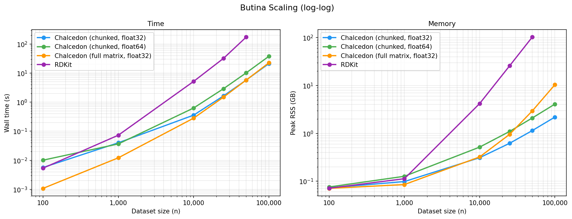
Wall time (s):
| n | Chalcedon (chunked, float32) | Chalcedon (chunked, float64) | Chalcedon (full matrix, float32) | RDKit |
|---|---|---|---|---|
| 100 | 0.006 | 0.010 | 0.001 | 0.005 |
| 1,000 | 0.040 | 0.037 | 0.012 | 0.073 |
| 10,000 | 0.357 | 0.628 | 0.281 | 5.160 |
| 25,000 | 1.640 | 2.910 | 1.490 | 32.150 |
| 50,000 | 5.750 | 10.180 | 5.740 | 172.820 |
| 100,000 | 21.140 | 37.720 | 22.490 | OOM |
Peak RSS (GB):
| n | Chalcedon (chunked, float32) | Chalcedon (chunked, float64) | Chalcedon (full matrix, float32) | RDKit |
|---|---|---|---|---|
| 100 | 0.08 | 0.08 | 0.07 | 0.08 |
| 1,000 | 0.11 | 0.14 | 0.09 | 0.12 |
| 10,000 | 0.33 | 0.55 | 0.35 | 4.50 |
| 25,000 | 0.67 | 1.18 | 1.02 | 27.70 |
| 50,000 | 1.23 | 2.25 | 3.16 | 110.40 |
| 100,000 | 2.35 | 4.39 | 11.17 | OOM |
At small dataset sizes, the Chalcedon (full matrix) implementation is fastest and all four methods show similar memory consumption. As datasets scale, the RDKit implementation becomes significantly slower and consumes more memory than the Chalcedon methods. RDKit and Chalcedon (full matrix) scale quadratically in memory, while the Chalcedon (chunked) methods scale roughly linearly. The float64 implementation roughly doubles the float32 implementation in both wall time and peak RSS.
Cutoff sweep
We ran each method using cutoffs spanning 0.3–0.9 on our 25k subset and found discrepancies in the resulting clusters at some cutoffs. These discrepancies are due to precision differences and the algebraic rearrangement of the cutoff comparison, as floating-point arithmetic can yield different results despite mathematical equivalence. While the methods are not bitwise identical at every cutoff, the discrepancies are very small where they exist (≤ 2.5% of cluster count).
Number of clusters:
| cutoff | Chalcedon (chunked and full matrix, float32) | Chalcedon (chunked, float64) | RDKit |
|---|---|---|---|
| 0.30 | 22,841 | 22,841 | 22,883 |
| 0.40 | 19,377 | 19,310 | 19,310 |
| 0.70 | 2,983 | 3,059 | 2,991 |
BitBIRCH-Lean comparison
As a challenge, we benchmarked Chalcedon's exact Butina ( time) against BitBIRCH-Lean, an approximate hierarchical clustering algorithm based on the BIRCH algorithm (≈ time). Unsurprisingly, BitBIRCH-Lean pulls away on both wall time and peak memory as dataset sizes increase, but Chalcedon remains comparable and a practical choice at these sizes while producing exact Butina clusters.
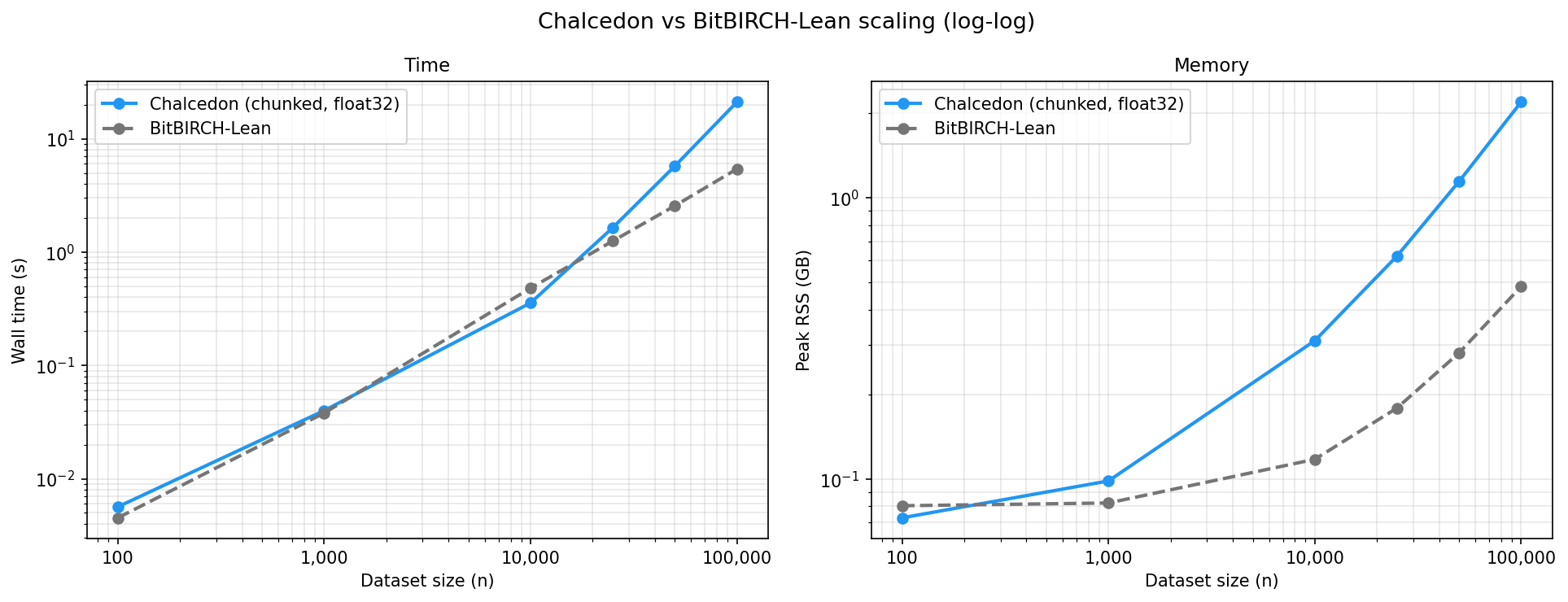
Wall time (s)
| n | Chalcedon | BitBIRCH-Lean |
|---|---|---|
| 100 | 0.006 | 0.005 |
| 1,000 | 0.040 | 0.038 |
| 10,000 | 0.357 | 0.482 |
| 25,000 | 1.640 | 1.250 |
| 50,000 | 5.750 | 2.560 |
| 100,000 | 21.140 | 5.420 |
Peak RSS (GB)
| n | Chalcedon | BitBIRCH-Lean |
|---|---|---|
| 100 | 0.08 | 0.09 |
| 1,000 | 0.11 | 0.09 |
| 10,000 | 0.33 | 0.13 |
| 25,000 | 0.67 | 0.19 |
| 50,000 | 1.23 | 0.30 |
| 100,000 | 2.35 | 0.52 |
As they are fundamentally different clustering algorithms, the two methods produce different partitions even at the same nominal threshold (BitBIRCH-Lean's similarity threshold set to 1 − cutoff to match Chalcedon's distance cutoff).
Number of clusters:
| n | Chalcedon (chunked, float32) | BitBIRCH-Lean |
|---|---|---|
| 100 | 95 | 98 |
| 1,000 | 678 | 866 |
| 10,000 | 3,107 | 7,382 |
| 25,000 | 5,058 | 16,318 |
| 50,000 | 7,067 | 29,140 |
| 100,000 | 9,590 | 51,232 |
How to use Chalcedon
Install from PyPI: uv pip install chalcedon.
For our recommended use case, the algorithm can be run directly from SMILES, with Morgan fingerprints (radius 2, 2048 bits, float32) computed internally.
import chalcedon

smiles = [
    "CCO",
    "c1ccccc1",
    # ...
]

splits = chalcedon.butina_split(
    smiles,
    fractions={"train": 0.8, "val": 0.1, "test": 0.1},
    cutoff=0.65,
    dtype="float32",  # or np.float32
)

train_smiles = splits["train"]
val_smiles = splits["val"]
test_smiles = splits["test"]
For full customizability, drop down to butina_cluster with your own fingerprints or descriptors. We recommend float64 for non-binary descriptors.
import numpy as np
import chalcedon

descriptors = my_descriptor_generator(molecules)  # numpy.ndarray of shape (n, d)

cluster_ids = chalcedon.butina_cluster(descriptors, cutoff=0.45, dtype="float64")
splits = chalcedon.greedy_cluster_split(
    cluster_ids,
    fractions={"train": 0.8, "val": 0.1, "test": 0.1},
)

train_indices = splits["train"]  # numpy.ndarray of indices into `descriptors`
Source code for the Chalcedon package and for reproducing our experiments can be found on GitHub. If there are other clustering algorithms you think we should include, or if you find bugs, please reach out to us at contact@rowansci.com or leave an issue on the GitHub repo.