How to Simulate Materials with DFT
by Raphael Stone · May 28, 2026

The Expulsion of Heliodorus from the Temple, Raffaello Sanzio (c. 1511–1512)
Welcome to the world of materials simulation, where reciprocal space is the conceptual norm, basis sets are described by a single number, and your "molecule" is infinite. Plane-wave density-functional theory (DFT) is the realm of the materials scientist, and while the nomenclature differs from molecular DFT, most of the underlying theory is the same. This post is an introduction to the machinery of plane-wave DFT.
Conceptual shifts
Plane-wave DFT is used to simulate any system with translational periodicity. The unit cell tiles space infinitely in every direction, which is key to the physics. Plane waves are sinusoidal, orthogonal, and space-filling, which makes them the natural basis for an infinite periodic solid.
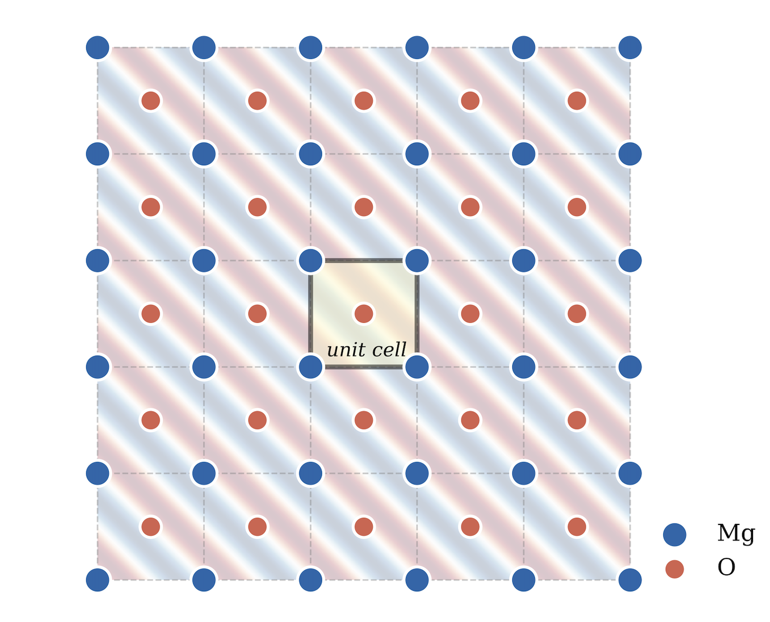
Figure 1: MgO infinite periodic solid
From this basis, there are a few practical consequences:
- To reduce computational cost, core electrons are almost always replaced with an effective potential.
- The number of plane waves included directly impacts the accuracy of your calculation.
- The crystal's electronic structure must be sampled at enough points for accuracy.
- The conductivity of the material being simulated can impact all of these choices.
We set some reasonable defaults so you don't have to worry about these choices if you don't want to. But it's always good to know why and how these decisions are made. I'll outline how you can approach these new concepts when simulating your materials.
Pseudopotentials
Core electrons are chemically inert. They don't participate in bonding, don't change between environments, and sit close to the nucleus where their wavefunctions oscillate rapidly. That rapid oscillation is expensive in a plane-wave basis. Pseudopotentials, unique to each element, solve this by replacing the core electrons and the nuclear potential with a single smooth effective potential that reproduces the correct behavior outside the core region. The valence electrons, meanwhile, are treated explicitly since they are responsible for bonding, conductivity, and reactivity. The expensive core physics gets absorbed into a potential, and the cheaper valence electrons are explicitly modeled.
There are three types of pseudopotentials in common use: norm-conserving, ultrasoft, and projector-augmented wave (PAW). Norm-conserving pseudopotentials make the least presumptive approximations at the core boundary, and are often a safe general-purpose choice. Ultrasoft pseudopotentials relax that boundary condition for efficiency, which works well for most main-group elements and oxides where the core isn't chemically active. PAW pseudopotentials take a different approach entirely. Rather than discarding the core, they retain enough information to reconstruct the full electron density near the nucleus. This is necessary for transition metals and properties like magnetic moments that are sensitive to what's happening in the core region.
The Standard Solid-State Pseudopotentials (SSSP) library is a curated, benchmarked set of pseudopotentials covering the first 103 elements of the periodic table. SSSP is a carefully chosen mix of norm-conserving, ultrasoft, and PAW pseudopotentials selected per element for accuracy and efficiency. We offer four SSSP variants: efficiency and precision (for speed and accuracy respectively), each available with PBE or PBEsol pseudopotentials. The pseudopotential variant should match your functional. Use PBEsol pseudopotentials only with the PBEsol functional, and PBE pseudopotentials with everything else.
Plane-wave basis
The plane-wave basis is controlled by two kinetic-energy thresholds: one for the wavefunctions (plane-wave cutoff) and one for the charge density (charge-density cutoff). All plane waves with kinetic energy below the relevant threshold are included in the basis. More plane waves means a more complete basis, higher accuracy, and more expense. The two cutoffs are typically related, but different pseudopotential types have different relationships between them.
Each pseudopotential dictates its own plane-wave cutoffs. Through convergence testing, published pseudopotentials have recommended cutoffs so the user can be confident their simulation is appropriately converged. Since these cutoffs are element-specific, they are tied to their corresponding pseudopotentials. The most demanding element in the structure sets the bar for the whole calculation. By way of example, consider MgO: while magnesium may converge at a plane-wave cutoff of 15 Eh for a given pseudopotential, oxygen may require 25 Eh, so the overall MgO plane-wave cutoff must be 25 Eh or higher.
We automatically set these recommended cutoffs for you, making running a Li(Ni1/3Mn1/3Co1/3)O2 calculation just as easy as running diamond. You don't have to sift through pseudopotential files, matching levels of theory and types before choosing your cutoffs. We give you the recommended minimum cutoff, and you can adjust it as you see fit. Generally, only raise the number from the suggested value.
To test if your energy cutoff is right, run the same calculation at increasing cutoffs and choose a cutoff that gets an error you're comfortable with. Below are convergence curves for silicon, copper, and MgO, with the recommended defaults in Rowan marked. In each case, the recommended value sits comfortably in the converged regime.
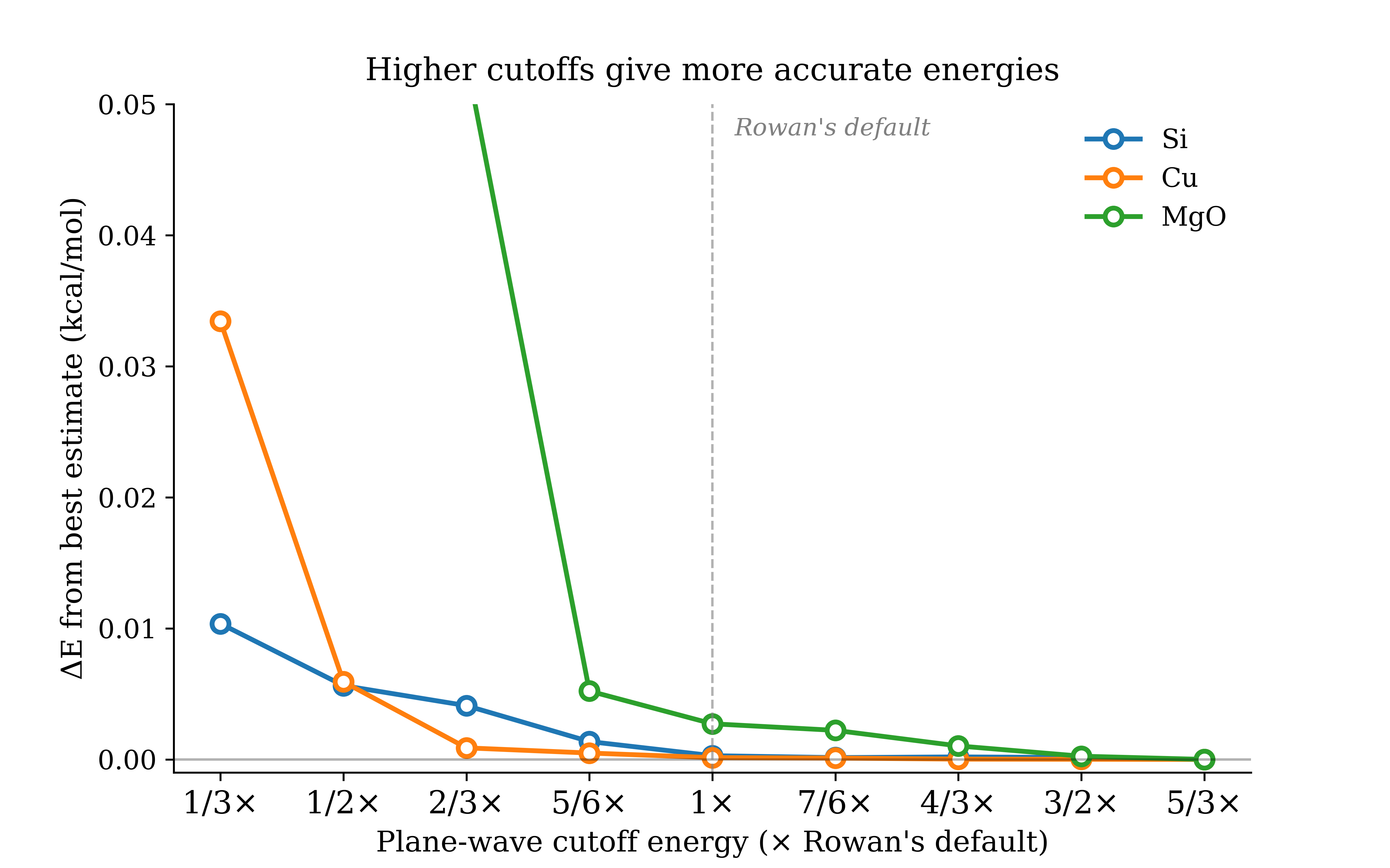
Figure 2: Energy vs. plane-wave cutoff convergence for Si, Cu, and MgO.
K-points and smearing
In a periodic solid, the electronic structure varies across reciprocal space and must be sampled on a grid. K-points are the sample locations on that grid. More k-points means a finer grid, higher accuracy, and more expense.
For insulators and semiconductors, the electronic structure varies smoothly across reciprocal space, and a coarse grid captures it faithfully. Metals are different. Filled and empty electronic states are separated by no band gap — they meet at a single energy. As a result, a given state can get counted as filled or empty with just a small change in how you sample. A coarse k-grid will undersample that boundary, leading to erratic convergence and unreliable energies.
The standard fix is smearing. Rather than enforcing a sharp step-function occupation at the Fermi level, you broaden it slightly into a smooth function, which stabilizes the k-point integration. Marzari–Vanderbilt cold smearing is the standard choice for metals.
We set k-point grids based on a target density in reciprocal space, calculated from your input cell geometry. As a result, smearing is left at the discretion of the user. Below are convergence curves for silicon, copper, and MgO with Rowan's default k-grid marked.
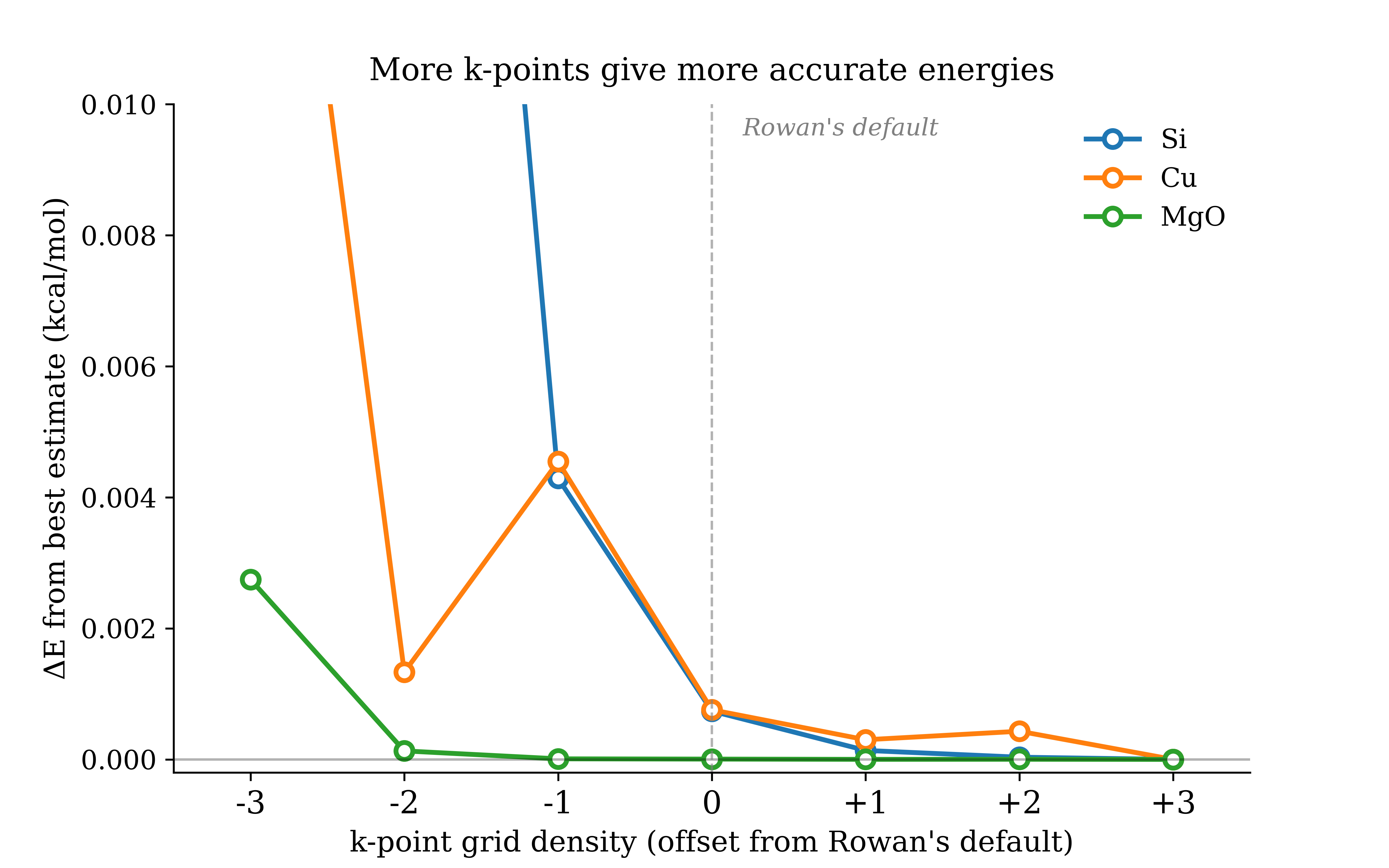
Figure 3: Energy vs. k-point density convergence for Si, Cu, and MgO
The poor convergence for copper is a cautionary tale. As previously mentioned, metals deserve extra attention. Namely, a denser k-point grid and applied smearing of ≈0.01 Eh. It is recommended to find literature values for materials similar to what you are simulating.
Further challenges
As you get acquainted with plane-wave DFT, it's worth appreciating some of the gentle quirks and engineering challenges.
Consider what happens when you try to remove an electron from your periodic system. In molecular DFT, this is a routine operation: you drop the electron count by one, solve, and report the cation energy. In periodic DFT, your unit cell is one tile of an infinitely repeating pattern. Removing an electron from the cell means removing one from every cell. You've created an infinite expanse of charged matter, and its Coulomb energy doesn't converge.
The standard workaround is to keep the cell electrically neutral by sleight of hand: compensate the missing electron with a fictitious uniform background charge, a smooth jellium smeared across the cell. The infinite-lattice problem dissolves and the calculation runs. But you haven't computed quite what you wanted. You've computed your charged species sitting in a sea of compensating charge, with its periodic images doing the same in every neighboring cell.
These sorts of problems each have unique solutions that require careful implementation. We hope to address many of these as we continue to build our capabilities for materials modeling.