Pocket Detection via Spamming Cofolding
by Ishaan Ganti · November 20, 2026

Millinery Shop by Perkins Harnly.
Computationally determining where a ligand can bind to a protein is an important step in drug discovery. Pocket-detection methods try to identify these druggable sites.
A little over a month ago, a preprint from Genesis Molecular AI introduced zPocket, a set of pocket-prediction heads trained on top of frozen cofolding features. The premise is that cofolding model embeddings already encode useful information about binding-site locations, and the zPocket results support this! But we were curious about how much of that embedded information we could recover through a simpler approach: repeatedly cofolding different ligands with the same protein.
We suspected that different ligands might bring out different binding-site preferences learned by the model. A cofolding model proposes a joint protein–ligand structure, even when the ligand might not actually bind. For pocket detection, this is probably an advantage over physics-based methods: the proposed placements may still have useful information about where the protein accommodates binders.
This approach ended up working quite well. On the proteins tested here, spamming cofolding recovered more annotated pockets than standalone zPocket, as well as zPocket + P2Rank, per the N+2 pocket recovery metric used in the paper.
The Method
We cofolded the same 16 ligands with each protein using Boltz-2, with no target-specific ligand selection, pocket-location hints, or experimental templates. General physical potentials were enabled, but there were no pocket-specific restraints. We had GPT-6 Astra select the panel to span different molecular shapes and functional groups.
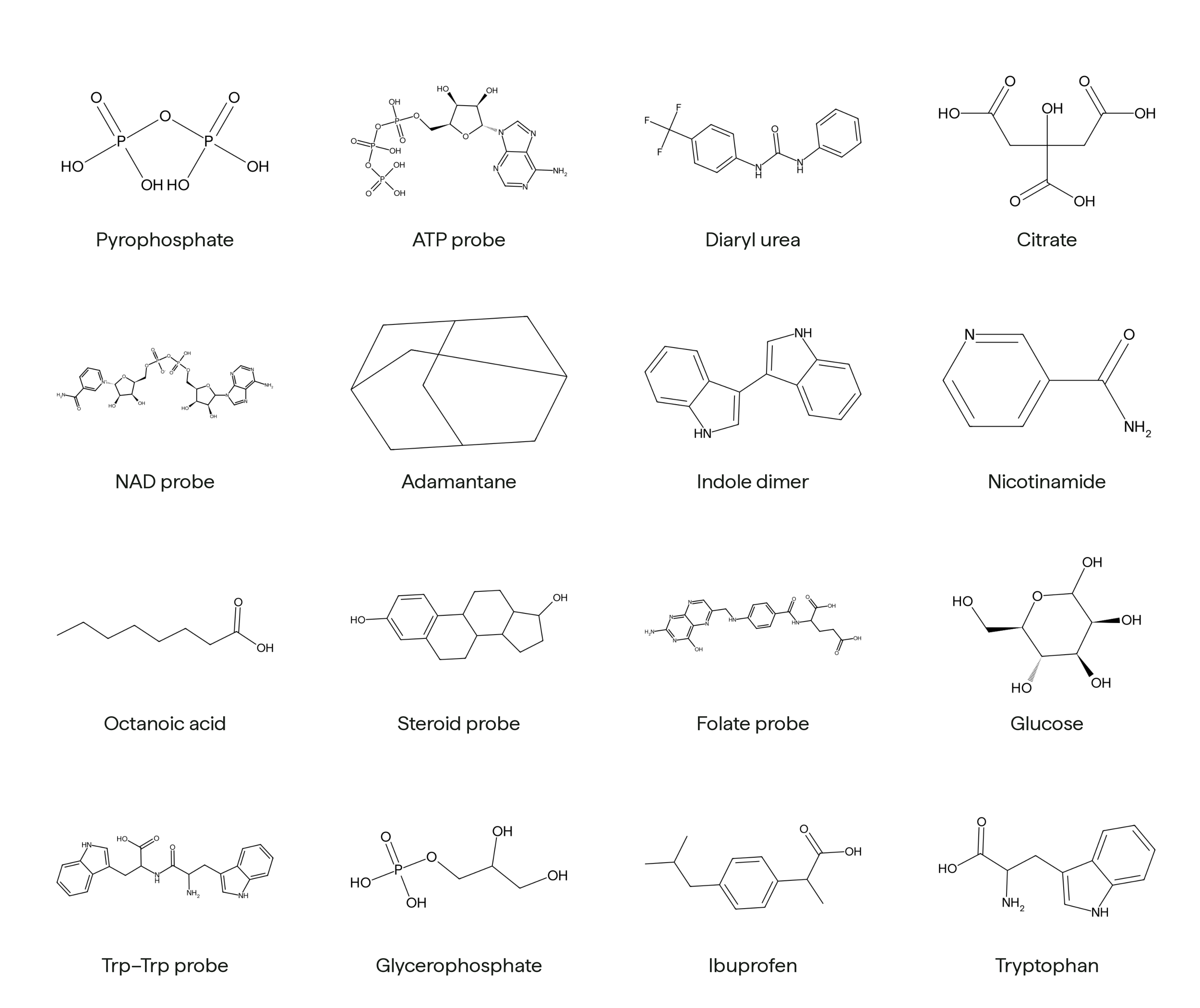
The selection of ligand probes, picked by GPT-6 Astra. The panel was chosen for chemical variety, as well as decent pocket discovery performance on a subset of the PocketWatch proteins.
The protein sequence and source MSA stayed the same across the 16 runs, but the predicted protein shape could change. To combine the placements, we aligned each predicted pose to a common predicted protein reference using residues near the ligand.
Each pocket suggestion was centered on the ligand heavy atoms within 4.5 Å of the protein. The distance restriction prevented long ligand tails from pulling the suggested center away from the contact region. If no ligand atoms met that cutoff, we used the generic ligand center.
We discarded probe placements with local alignment RMSD above 5 Å, then ranked the remaining suggestions by multiplying ligand ipTM and mean ligand-heavy-atom pLDDT. Finally, we removed any suggestion within 4 Å of an already retained, higher-ranked center.
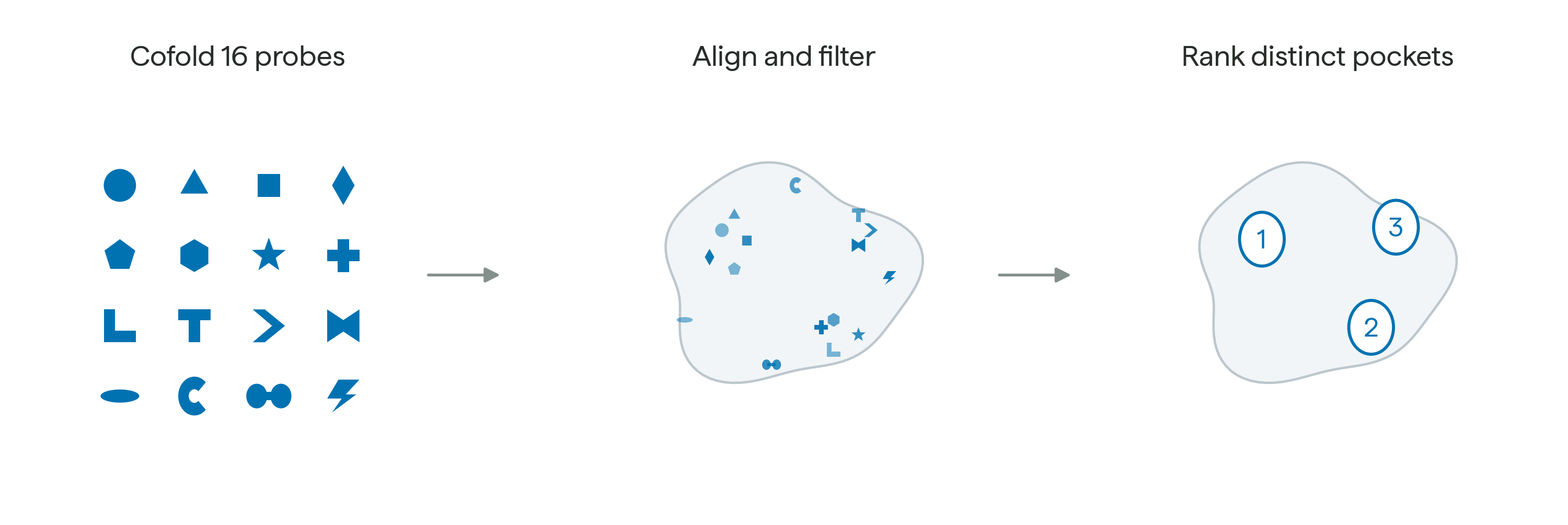
A schema of the method. Each symbol represents a different probe.
It's worth noting that these experiments don't isolate the benefit of probe diversity from that of repeated cofolding. One could test this by comparing the 16-probe panel with 16 runs of a single probe using different random seeds.
Comparisons
We developed the probe workflow using an initial protein set and report paired results for 70 of those proteins, alongside 140 additional proteins. The combined comparison covers 210 proteins and 255 annotated sites; Appendix A reports the two groups separately.
The 255 annotated sites come from PocketWatch, which derives binding-site labels from experimentally observed protein–ligand structures in the Protein Data Bank. These annotations provide experimental support for the known sites, but they aren't exhaustive! A prediction that misses the annotations therefore isn't necessarily a poor prediction; the site might just be unannotated. Appendix C details the protein selection more thoroughly.
We compared the probe method with standalone zPocket and a P2Rank + zPocket hybrid. zPocket assigns a score to each protein residue, then groups nearby high-scoring residues into pocket suggestions. P2Rank searches the protein's shape for cavities. The hybrid keeps suggestions from both sources and uses zPocket's residue scores to rank them. So, it can propose cavities that just zPocket's grouping step misses.
All results below use the same predicted protein structure: the ESMFold2 fold used by zPocket and P2Rank. We overlaid the saved cofolded probe placements into that structure's coordinate frame after inference. Notably, no method used an experimental structure as its prediction reference. There are some annoyances that come with this, discussed in Appendix B.
For a protein with N annotated sites, we evaluate up to its N+2 highest-ranked eligible suggestions. A site is recovered if any of those suggestions lies within 4 Å of its annotated center. Following the paper's metric, sites are scored independently, so one suggestion can recover more than one nearby site.
Results
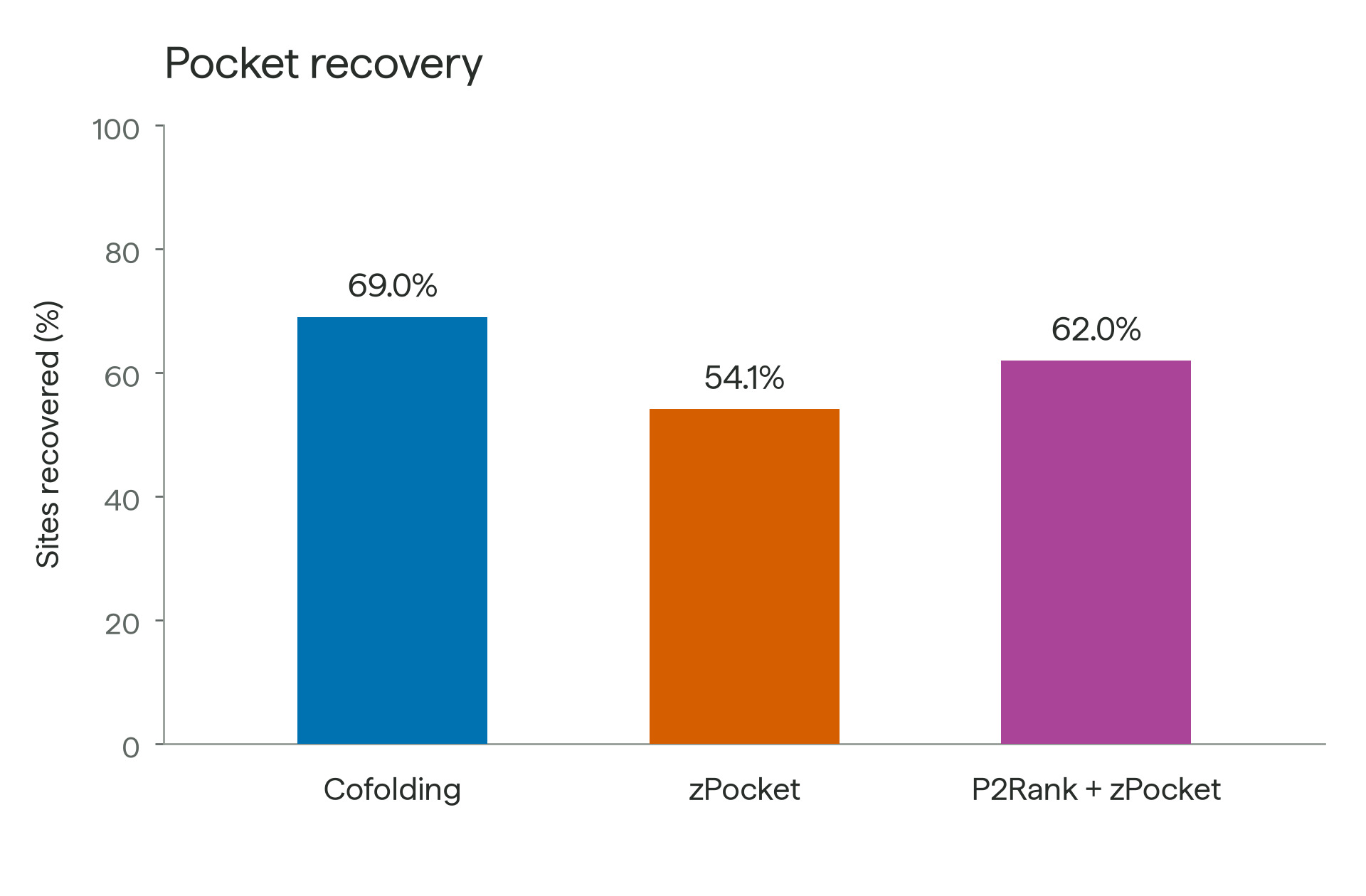
Pocket recovery across 210 proteins and 255 annotated sites using the paper's N+2 allowance. Cofolding, zPocket, and P2Rank + zPocket supplied 614, 216, and 639 eligible pocket suggestions, respectively.
Cofolding recovered 176 of 255 sites (69.0%), compared with 138 (54.1%) for zPocket and 158 (62.0%) for the hybrid. Cofolding and the hybrid supplied similar numbers of suggestions (614 and 639, respectively), while standalone zPocket returned much shorter lists (216 suggestions total).
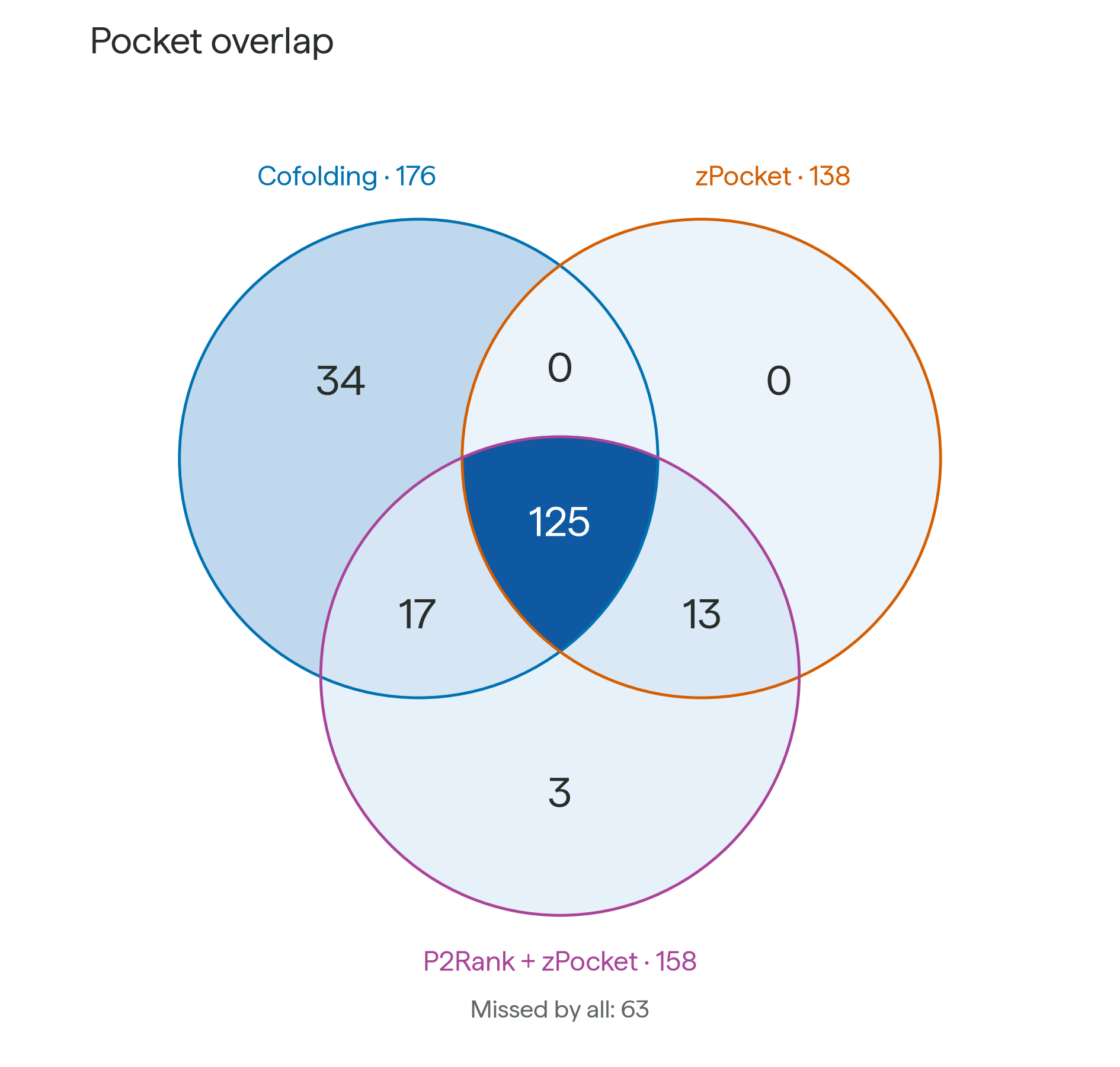
Pocket site recovery overlap between the three methods. Cofolding provides a decent amount of new signal compared to the zPocket-based methods, but most of the signal is shared between all three methods.
Together, the methods recover 192 of 255 sites (75.3%). Cofolding finds 34 sites missed by both baselines; the baselines find 16 sites missed by cofolding. All three recover 125 sites. The strong central overlap likely has to do with all three methods loosely being based on cofolding models—or some pockets just being obvious—but this is just a guess.
Here's an example of cofolding results from a PocketWatch protein with two annotated sites:
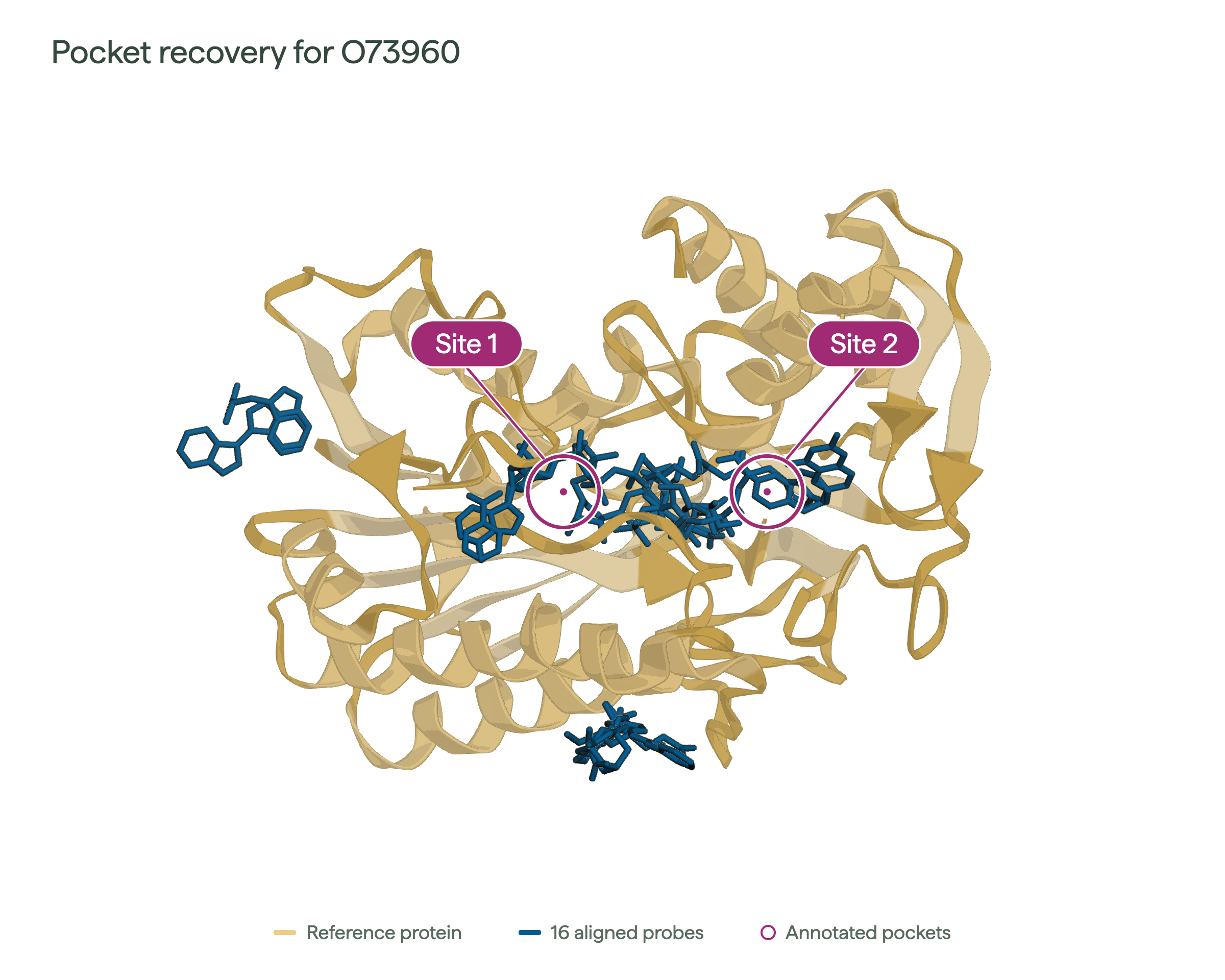
All 16 independently cofolded probes (blue) are aligned to the reference protein. Plum circles mark annotated sites. The two annotated sites for this protein were recovered by the first and third pocket predictions, satisfying the N+2 metric.
Broader Thoughts
LLMs can now do a ton of protein analysis by themselves when given access to pretty barebones Python sandboxes. We've seen this at Rowan through several mini-benchmarks we've run (for example, this binder optimization study and this LLM-guided inverse folding benchmark).
Cofolding models let LLMs change ligands, focus on specific regions, and impose contact constraints. The appeal here is that pocket finding can use those capabilities directly, without training a separate pocket-prediction head. New cofolding models can therefore be tested with the same basic probe workflow.
It's entirely possible to make specialized predictors more steerable, too, but the point is we may not need to allocate research projects to this if cofolding probes work well.
We suspect a useful combination will be fast pocket predictions for broad screening and adaptive cofolding for closer investigation of individual proteins. Running 16 cofolding jobs is more computationally expensive than running the ESMFold2–zPocket pipeline once per protein, though one could reasonably try decreasing the number of probes.
Appendix
A. Separated Results
The initial pipeline was fixed before evaluating the 140 additional proteins. The plots below apply the final processing choices consistently to both groups.
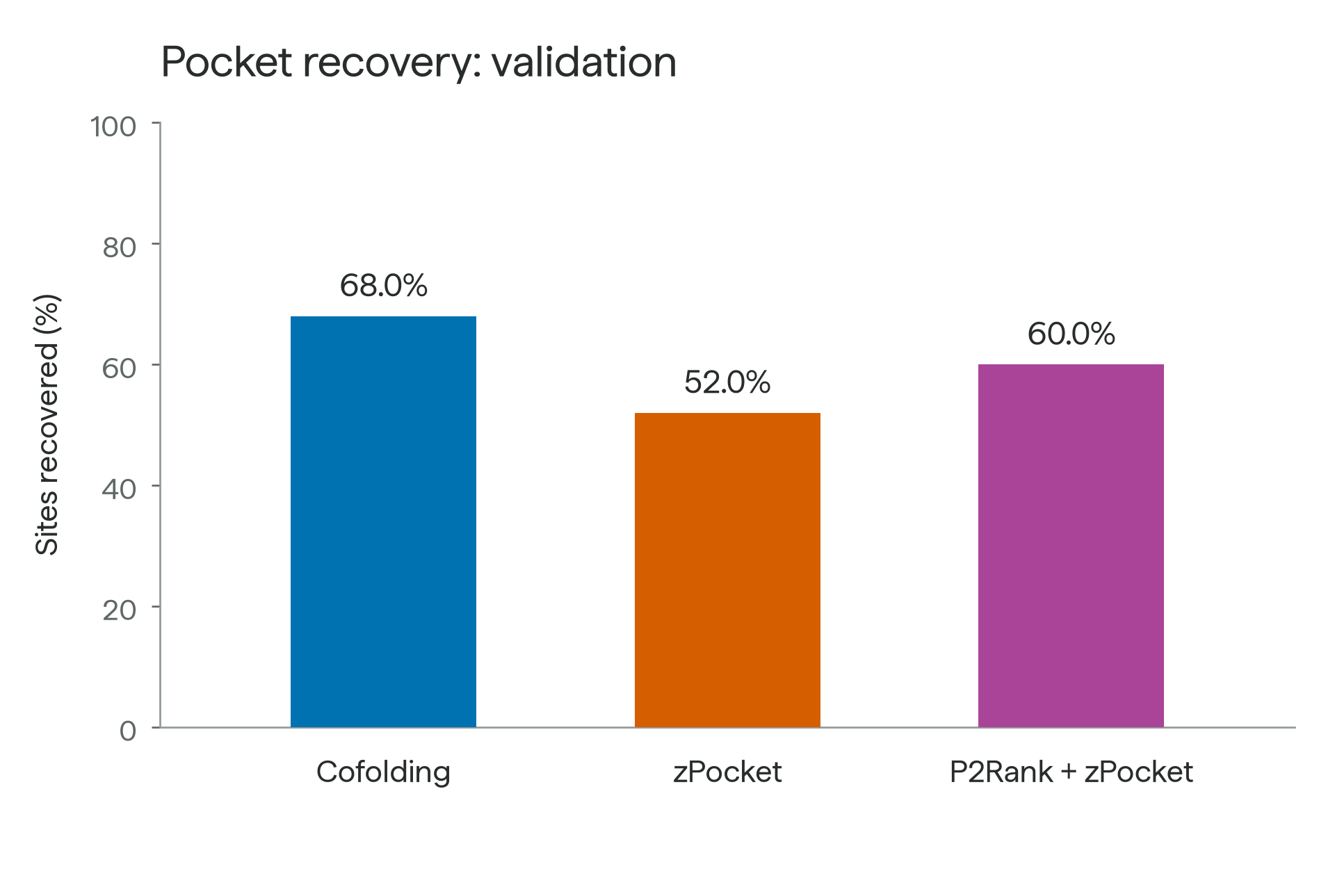
Results on just the "validation" set, using the N+2 metric.
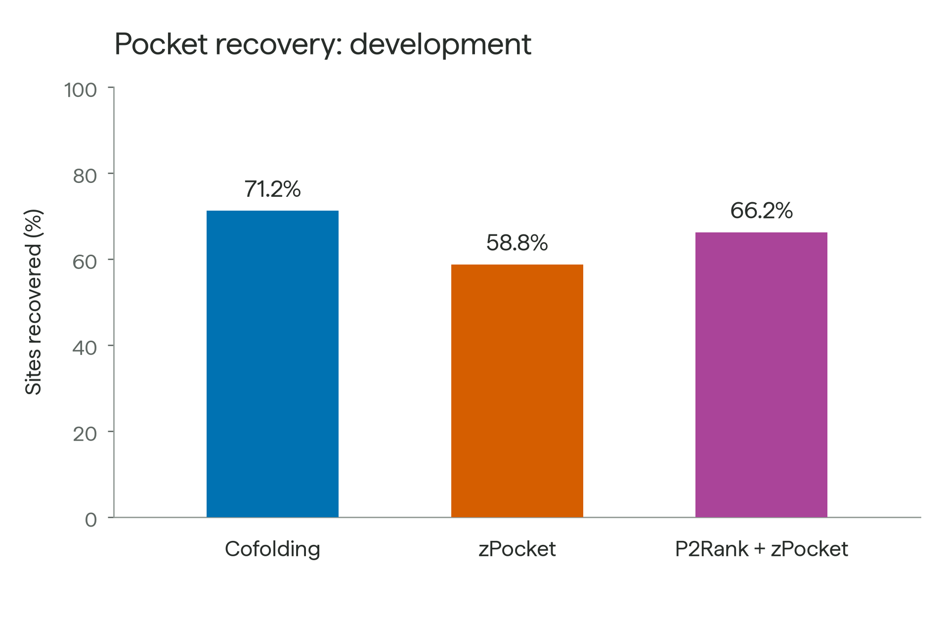
Results on just the "development" set, using the N+2 metric.
B. Reference Structures and Local Alignment
zPocket uses internal features from ESMFold2 to assign a pocket score to each residue. It then uses the predicted protein structure to group nearby high-scoring residues into pocket suggestions. P2Rank also uses this structure to identify cavities.
We used Boltz-2 for probe cofolding and ESMFold2 for the baselines. Initially, we aligned probes to the predicted structures distributed with PocketWatch. Here, we use the exact ESMFold2 structures from our zPocket runs, putting all methods' predictions in the same coordinate frame.
Astute readers might notice that we used Boltz-2 for our probe method and that using ESMFold2 would have likely been more consistent. This is correct!
For each probe, we select protein residues with a heavy atom within 5 Å of the ligand. We match their Cα atoms to the corresponding residues in the reference, then rotate and translate the cofolded structure to minimize their RMSD. The probe moves with that transformation. We fit the nearby residues rather than the entire protein so that distant domain movements don't dominate alignment error.
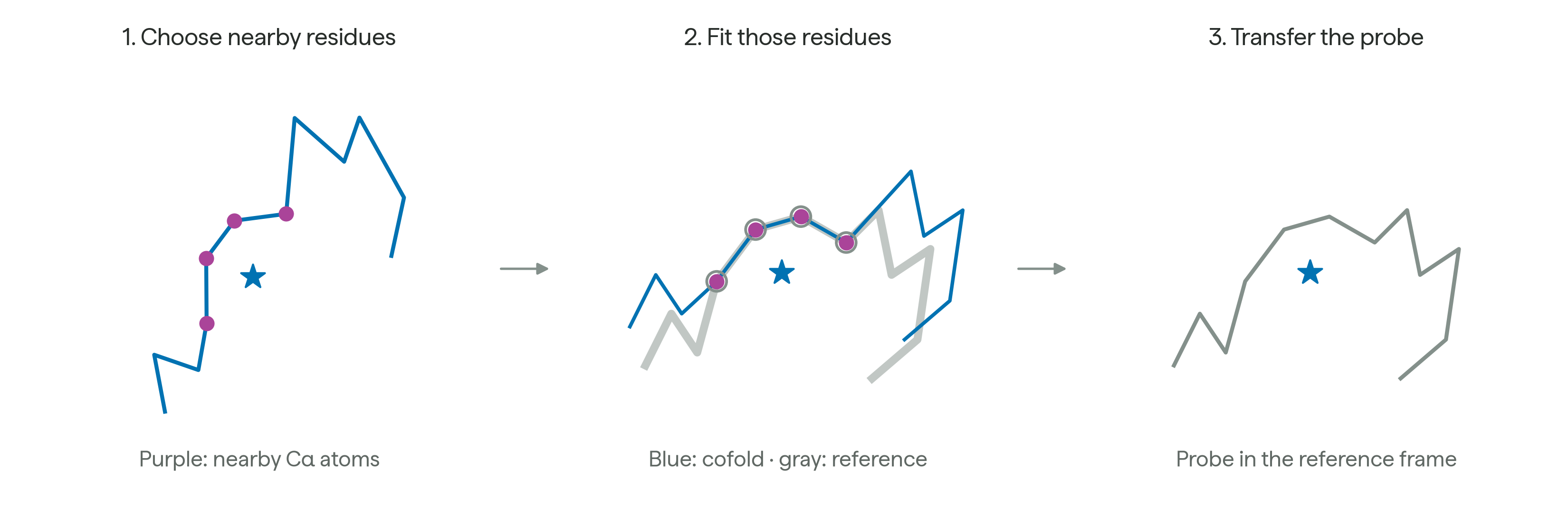
This works when the local protein shapes are sufficiently similar. If the pocket opens, closes, or rearranges between structures, a rigid alignment cannot reconcile the difference. Such differences can reflect either real protein flexibility or some sort of prediction error.
We require at least three noncollinear anchor residues and a local alignment RMSD of at most 5 Å. Together, these checks reject 272 of 2,240 validation placements. Three proteins lose all 16 placements but remain in the evaluation, contributing zero recovered sites.
There's also a separate uncertainty in PocketWatch's answers. Experimental ligands were observed in experimental protein structures, but we score predictions on the ESMFold2 reference. PocketWatch maps those known ligand locations onto the predicted structure by aligning the surrounding residues. If those local shapes differ, the transferred answer location can be uncertain.
Using the same reference makes the three methods' coordinates more comparable. It still fails to eliminate errors in the predicted structure, of course, or in PocketWatch's transferred labels. And, the annotations may omit real binding sites. However, these are shared benchmark limitations.
C. Data Selection
We built the dataset in stages. We started with around 32 short proteins (80–180 residues) to keep repeated cofolding experiments manageable while designing the processing pipeline. Then, we added batches spanning different protein lengths, eventually bringing the development set to 70 proteins.
We expanded the evaluation with 140 additional proteins: 40 selected for sequence diversity and coverage across protein lengths, and 100 sampled from the remaining eligible proteins. For the latter, we sorted proteins by length, divided them into ten nearly equal-sized groups, and selected ten per group using a random ordering. The 40-protein set was deliberately balanced across protein lengths, sequence diversity, and annotated pocket counts by GPT-6 Astra. The 100-protein set was sampled randomly within length groups. Importantly, neither selection used prediction results.
Together, these batches cover 210 PocketWatch proteins containing 255 annotated sites. Note that the preference for short proteins in the development set makes the combined set biased in this direction with respect to PocketWatch.
D. Alternative Performance Evaluation
At Rowan, we like to think about how experiments like this one translate to workflows. In this case, we consider a pocket-detection workflow. It's instructive to list a few qualities we'd hope such a workflow possesses:
- The ability to recover, with very high ranking, at least a single good pocket on a target.
- Some proxy for how stable or prominent a given pocket is.
- The ability to effectively filter out false positives!
Of these wishes, simultaneously optimizing for the first and third is probably how we'd go about building a pocket-detection workflow. However, the N+2 metric doesn't really measure the signal we'd want to do this. For example, a method applied to a protein with just a single binding site could produce three sites. If the first two aren't actually binding sites but the third is, the N+2 metric would deem this detection result a pass. But users of this workflow would understandably be likely to dock their ligands into one of the first two pockets, leading to incorrect downstream computations.
In this line of thinking, we think a complementary metric is whether the top-ranked site is actually a recognized site. While definitely not a holistic metric on its own, it addresses aspects of the aforementioned issue with the N+2 metric. Here are the corresponding success rates by method:
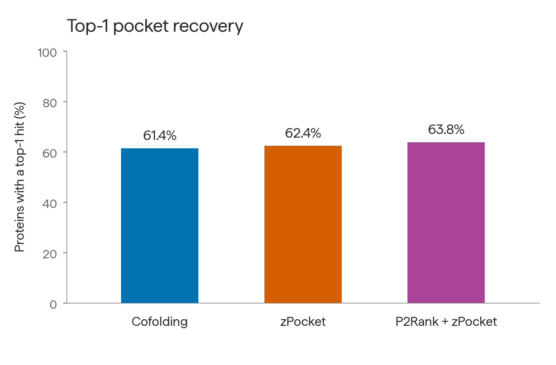
Top-1 recovery across 210 proteins with annotated pockets. A hit requires the first suggestion to lie within 4 Å of an annotated center.
All methods do very similarly here, with cofolding just getting edged out by the zPocket-based methods.
All data produced while writing this blog post are available here. Thanks to Corin Wagen, Nate Gruver, and Zachary Fried for reading drafts of this and providing helpful comments.